A Step-by-Step Guide to NMR-Based Plant Metabolomics: From Sample Prep to Data Analysis for Biomedical Research

Abstract

This comprehensive guide provides researchers, scientists, and drug development professionals with a detailed workflow for NMR-based plant metabolomics. We cover the foundational principles of NMR spectroscopy for metabolite profiling, a complete step-by-step methodological pipeline from tissue harvest to spectrum acquisition, common troubleshooting and optimization strategies for data quality, and validation protocols including comparisons to mass spectrometry. This article serves as a practical handbook for unlocking the chemical diversity of plants for biomarker discovery and natural product development.

Understanding NMR in Plant Metabolomics: Core Principles and Strategic Advantages

Application Notes

Nuclear Magnetic Resonance (NMR) spectroscopy is a powerful, non-destructive analytical technique that provides a comprehensive snapshot of the metabolome. Its quantitative nature, minimal sample preparation, and ability to identify novel compounds make it exceptionally suitable for untargeted profiling of complex plant extracts. NMR excels in detecting a wide range of primary and secondary metabolites (e.g., alkaloids, phenolics, terpenes, sugars, organic acids) simultaneously, with high reproducibility. It is the cornerstone for metabolomics studies aiming to understand plant physiology, response to stress, or the discovery of bioactive compounds for drug development.

Key Advantages Quantified

Table 1: Comparative Advantages of NMR in Plant Metabolomics

Feature	NMR Spectroscopy	Alternative (e.g., LC-MS)
Sample Preparation	Minimal; often just dissolution in deuterated solvent.	Extensive; requires extraction optimization, filtration, derivatization possible.
Destructiveness	Non-destructive; sample recoverable for further analysis.	Destructive; sample consumed.
Quantitation	Absolute, without need for compound-specific standards.	Relative, requires pure standards for absolute quantitation.
Reproducibility	Very High (CV < 2%).	Moderate to High (CV 5-20%).
Structural Elucidation	Direct, provides detailed atomic connectivity.	Indirect, relies on fragmentation patterns and libraries.
Throughput	Moderate (5-20 min/sample for 1D).	High (short LC runs).
Detectable Dynamic Range	Limited (~10^3).	Very wide (~10^5-10^6).
Key Strength	Structural unknowns, quantitation, reproducibility.	Sensitivity, throughput, wide coverage.

Table 2: Typical Metabolite Classes Detected by NMR in Plant Extracts

Chemical Shift Range (1H, ppm)	Dominant Metabolite Class	Example Compounds
0.8 - 3.0	Aliphatic compounds	Fatty acids, terpenes, organic acids (e.g., citrate, succinate).
3.0 - 5.5	Sugars and Carbohydrates	Sucrose, glucose, fructose, polysaccharides.
5.5 - 8.5	Aromatics and Unsaturates	Phenolic acids, flavonoids, alkaloids, amino acids.
8.5 - 10.0	Aldehydes and Formyl groups	Certain alkaloids, vanillin derivatives.

Experimental Protocols

Protocol 1: Sample Preparation for Untargeted 1H-NMR Profiling of Plant Leaf Tissue

Objective: To reproducibly extract and prepare a polar metabolite fraction from plant leaf tissue for 1H-NMR analysis.

Materials: See "The Scientist's Toolkit" below.

Procedure:

• Harvest & Quench: Rapidly harvest ~100 mg of fresh plant leaf tissue using a cooled, pre-weighed ceramic mortar and pestle. Immediately freeze-quench the tissue in liquid nitrogen.
• Homogenization: Under continuous liquid N2 cooling, grind the tissue to a fine powder.
• Extraction: Transfer the powder to a pre-cooled 2 mL microcentrifuge tube. Add 1.5 mL of cold methanol:water (4:1, v/v) extraction solvent. Vortex vigorously for 30 seconds.
• Sonication: Sonicate the mixture in an ice-water bath for 15 minutes.
• Centrifugation: Centrifuge at 14,000 x g for 20 minutes at 4°C.
• Collection & Evaporation: Transfer the supernatant to a new glass vial. Dry the supernatant completely using a gentle stream of nitrogen gas or a vacuum concentrator.
• NMR Sample Preparation: Reconstitute the dried extract in 600 µL of phosphate buffer (pH 6.0, 100 mM) in D2O containing 0.5 mM TMSP-d4 (internal standard for chemical shift referencing and quantitation). Vortex and sonicate briefly to ensure complete dissolution.
• Clarification: Centrifuge the solution at 14,000 x g for 5 minutes to remove any particulate matter.
• Loading: Transfer 550 µL of the clear supernatant into a clean 5 mm NMR tube. The sample is now ready for data acquisition.

Protocol 2: Standard 1D 1H-NMR Data Acquisition

Objective: To acquire a quantitative 1H-NMR spectrum for untargeted metabolite profiling.

Materials: Prepared NMR sample, 500+ MHz NMR spectrometer equipped with a room-temperature or cryogenic probe.

Procedure:

• Temperature Equilibration: Insert the sample into the magnet and allow it to equilibrate to the probe temperature (typically 298K) for 5 minutes.
• Tuning & Locking: Tune and match the probe, then activate the deuterium lock on the D2O signal.
• Shimming: Perform automatic shimming routines (e.g., gradient shimming) to optimize magnetic field homogeneity.
• Pulse Sequence Selection: Use a standard 1D nuclear Overhauser effect spectroscopy (NOESY) presaturation pulse sequence (noesygppr1d on Bruker, noesygppr1d equivalents on other vendors) to suppress the residual water signal.
• Parameter Setup:
  • Spectral Width: 20 ppm (centered on water signal at ~4.7 ppm).
  • Number of Scans (NS): 128-256 for sufficient signal-to-noise.
  • Relaxation Delay (D1): 4 seconds.
  • Acquisition Time: ~3 seconds.
  • Total Experiment Time: ~10-15 minutes per sample.
• Data Acquisition: Run the experiment.
• Processing: Apply exponential line broadening (0.3 Hz), Fourier transformation, phase and baseline correction, and reference to TMSP-d4 at 0.0 ppm.

Visualizations

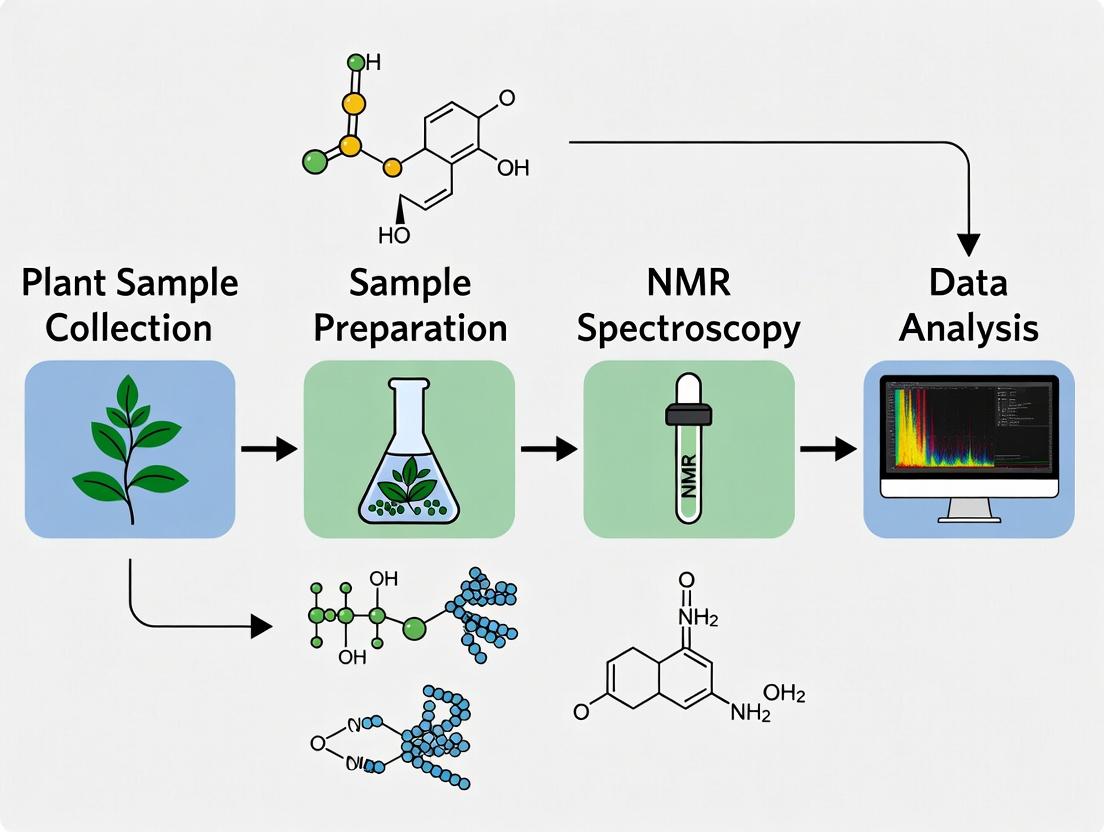
Workflow for Plant Metabolite NMR Profiling

Key NMR Advantages for Untargeted Profiling

The Scientist's Toolkit

Table 3: Essential Research Reagent Solutions for NMR-based Plant Metabolomics

Item	Function & Specification
Deuterated Solvent (D2O)	Provides the lock signal for the NMR spectrometer. High isotopic purity (99.9% D) is essential.
Deuterated Methanol (CD3OD)	Used for extraction or for preparing less polar NMR samples.
Potassium Phosphate Buffer (in D2O)	Maintains constant pH (e.g., pH 6.0), crucial for chemical shift reproducibility. Typically 50-100 mM.
Internal Standard (TMSP-d4)	Sodium 3-(trimethylsilyl)propionate-2,2,3,3-d4. Provides chemical shift reference (0.0 ppm) and enables quantitative concentration calculations.
Methanol (HPLC grade)	Primary component of extraction solvent for polar metabolites.
Liquid Nitrogen	For instantaneous quenching of metabolic activity and tissue homogenization.
Ceramic Mortar & Pestle	For grinding frozen tissue without introducing contaminants.
5 mm NMR Tubes	High-quality, matched tubes for consistent spectral line shape.
NMR Spectrometer	500 MHz or higher field strength equipped with an automated sample changer and a cryogenic probe for enhanced sensitivity.

Within a comprehensive thesis on NMR-based plant metabolomics, the selection of an analytical platform is paramount. Nuclear Magnetic Resonance (NMR) spectroscopy stands out due to its core advantages of providing inherently quantitative, non-destructive, and highly reproducible analysis. These characteristics make it an indispensable tool for longitudinal studies, quality control in phytopharmaceutical development, and the reliable biomarker discovery required by researchers and drug development professionals. This application note details protocols and experimental designs that leverage these advantages.

Quantitative Analysis: Absolute Metabolite Concentration Determination

NMR signal intensity is directly proportional to the number of nuclei generating it, enabling absolute quantification without compound-specific calibration curves.

Protocol: Absolute Quantification via PULCON

Principle: The Pulse Length-Based Concentration Determination (PULCON) method uses an external reference of known concentration to relate signal intensities between samples.

Materials & Procedure:

• Sample Preparation: Prepare plant extract (e.g., 50 mg dried leaf extracted in 600 µL D₂O-based phosphate buffer, pH 6.0, with 0.5 mM TMSP-d₄ as internal chemical shift reference).
• External Reference: Prepare a separate capillary or insert containing a known concentration (e.g., 10.0 mM) of DSS (4,4-dimethyl-4-silapentane-1-sulfonic acid) in D₂O.
• NMR Acquisition: Acquire ¹H NMR spectra for both the sample and the external reference under identical instrumental conditions (90° pulse width, receiver gain, temperature (298 K), and number of scans (128)).
• Data Processing: Apply identical processing parameters (exponential line broadening: 0.3 Hz, zero-filling, Fourier transform, phase, and baseline correction) to both spectra.
• Calculation: Use the formula: C_sample = (I_sample / I_ref) * (N_ref / N_sample) * (V_ref / V_sample) * C_ref Where I=integral, N=number of scans, V=excited volume, C=concentration.

Table 1: Quantitative Data from NMR Analysis of Mentha piperita Leaf Extract

Metabolite	¹H Chemical Shift (ppm)	Integral Value (Sample)	Integral Value (DSS Ref)	Calculated Concentration (mM)	± RSD (%) (n=5)
Alanine	1.48 (d)	15.2	25.0	4.21	1.8
Choline	3.21 (s)	8.7	25.0	2.41	2.1
Sucrose	5.41 (d)	5.5	25.0	1.52	2.5
DSS (Ref)	0.00 (s)	25.0	25.0	10.00	N/A

Non-Destructive Analysis: Live Tissue and Longitudinal Monitoring

The non-destructive nature of NMR allows for the analysis of intact tissues or the recovery of precious samples post-analysis.

Protocol: High-Resolution Magic Angle Spinning (HR-MAS) of Live Plant Tissues

Application: Metabolic profiling of intact plant biopsy samples (e.g., root nodules, leaf discs, fruit skin) to preserve spatial information and sample viability.

Methodology:

• Sample Handling: Excise a small, defined tissue segment (e.g., ~10 mg). Rinse briefly with D₂O to lock signal.
• Loading: Place the tissue into a disposable, zirconia HR-MAS rotor. Add 10 µL of D₂O containing TMSP for lock and reference.
• Spinning: Insert rotor into the HR-MAS probe. Spin at the magic angle (54.7°) at a rate of 4-5 kHz to eliminate line broadening from residual anisotropic interactions.
• Acquisition: Run a standard 1D ¹H NMR sequence with water suppression (e.g., presaturation). Temperature control at 4°C to slow metabolic degradation.
• Sample Recovery: After data acquisition, carefully remove the tissue from the rotor for subsequent morphological study, cultivation, or alternative analytical techniques (e.g., genomics).

Diagram Title: HR-MAS NMR Workflow for Non-Destructive Plant Analysis

Reproducible Analysis: Standardization for Multi-Center Studies

NMR offers exceptional instrument-to-instrument and day-to-day reproducibility, critical for large-scale metabolomic studies and clinical translation.

Protocol: Standardized NMR Metabolomics for Multi-Batch Plant Extracts

Goal: Ensure data consistency across multiple NMR instruments or over long study durations.

Detailed Workflow:

• Standard Operating Procedure (SOP):
  • Extraction: Precisely weigh 50.0 ± 0.1 mg dried powder. Add 1.00 mL of extraction solvent (CD₃OD:D₂O:KH₂PO₄ buffer in D₂O, 2:1:1, pH 6.0). Vortex 1 min, sonicate 15 min (20°C), centrifuge 15 min (13,000 rpm, 4°C). Transfer 600 µL supernatant to 5 mm NMR tube.
• Instrument Calibration: Prior to batch run, perform automated probe tuning/matching, lock gradient optimization, and 90° pulse width calibration for each sample. Use the same standard sample (e.g., 5 mM sucrose in buffer) to check line shape (resolution at 0.55 Hz) and sensitivity (S/N > 500 for reference peak).
• Automated Acquisition: Utilize a standardized, automated acquisition program (e.g., Bruker 'avance' or Jeol 'Delta'):
  • Pulse Sequence: 1D NOESYGPPR1D (for water suppression)
  • Parameters: Spectral width: 20 ppm, Offset frequency: 4.7 ppm (on water), Acquisition time: 4 s, Relaxation delay: 4 s, 90° pulse width: as calibrated, Number of scans: 128, Temperature: 298 K.
• Data Processing Automation: All FIDs processed identically:
  • Software: Use AMIX, Chenomx, or in-house scripts.
  • Steps: Apply 0.3 Hz exponential line broadening -> Zero-filling to 128k -> Fourier Transform -> Automatic phase correction -> Polynomial baseline correction (degree 3) -> Reference to TMSP at 0.0 ppm -> Bin data (0.01 ppm buckets) or perform targeted profiling.

Table 2: Inter-Day and Inter-Instrument Reproducibility Data

Metabolite	Intra-Day Precision (CV%, n=10)	Inter-Day Precision (CV%, n=5 days)	Inter-Instrument Precision* (CV%, n=3)
Alanine	1.2	2.5	3.8
Aspartate	1.5	2.8	4.1
Glucose	1.8	3.2	4.5
Succinate	1.0	2.1	3.5

*Instruments: 600 MHz (A), 500 MHz (B), 600 MHz (C) from different manufacturers.

The Scientist's Toolkit: Key Research Reagent Solutions

Table 3: Essential Materials for NMR-Based Plant Metabolomics

Item	Function & Rationale
D₂O (Deuterium Oxide)	Provides a field frequency lock signal for the NMR spectrometer; used as the primary solvent to minimize the huge ¹H solvent signal.
TMSP-d₄ (Trimethylsilylpropanoic acid)	Internal chemical shift reference (set to 0.0 ppm) and quantitative internal standard for ¹H NMR in aqueous solutions.
DSS (4,4-dimethyl-4-silapentane-1-sulfonic acid)	An alternative, non-volatile internal chemical shift and concentration standard, often preferred for its insensitivity to pH.
Phosphate Buffer (in D₂O, pD 6.0)	Maintains consistent pH across all samples, which is critical for reproducible chemical shifts of pH-sensitive metabolites (e.g., organic acids).
CD₃OD (Deuterated Methanol)	Organic solvent used in extraction solvent systems (e.g., methanol-water) for comprehensive metabolite recovery from plant tissue.
Zirconia HR-MAS Rotors	Disposable, inert sample holders for HR-MAS experiments, allowing high-speed spinning of semi-solid tissues.
Standard Reference Mixture (e.g., ERETIC2, EUROSPIN)	Electronic or physical reference sample used for absolute quantification and inter-instrument signal calibration.

Diagram Title: Core NMR Advantages Drive Key Metabolomics Applications

The trifecta of quantitative power, non-destructive capability, and unmatched reproducibility establishes NMR spectroscopy as a cornerstone methodology in plant metabolomics. The protocols and data presented here provide a practical, step-by-step framework for integrating these advantages into a research thesis, enabling robust, translatable findings for drug discovery and plant science.

In NMR-based plant metabolomics, meticulous pre-experimental planning is paramount. The biological question and the derived hypothesis form the foundational blueprint that dictates every subsequent step, from experimental design to data interpretation. A poorly defined question leads to inconclusive data, wasted resources, and compromised statistical power. This protocol details the systematic process of formulating a robust, testable biological question and hypothesis within the context of plant metabolomics research, ensuring the generated NMR data is meaningful and actionable.

Key Considerations and Quantitative Benchmarks

Table 1: Quantitative Benchmarks for Hypothesis Formulation in Plant Metabolomics

Consideration	Description	Typical Benchmark / Metric
Specificity	The precision of the variables (genotype, treatment, metabolite class).	Define at least 2-3 key metabolite classes (e.g., phenylpropanoids, alkaloids).
Measurability	The ability to quantify the response via NMR.	Target metabolites must have known, resolvable NMR signatures (e.g., aliphatic region δ 0.5-3.0, aromatic δ 5.5-9.0).
Biological Replicates	Number of independent biological samples per group.	Minimum n=6 for robust statistical power in metabolomics studies.
Technical Replicates	Number of repeated measurements from the same sample.	n=3 for NMR sample preparation (extraction to data acquisition).
Effect Size	The expected magnitude of metabolic change.	Hypothesis should predict a change >2-fold for key discriminant metabolites.
Statistical Power	Probability of detecting a true effect.	Aim for power (1-β) ≥ 0.8, with significance level α ≤ 0.05.

Application Notes and Detailed Protocols

Protocol 1: Defining the Biological Question

Objective: To transform a broad area of interest into a focused, actionable research question.

• Identify the Broader Context: Start with the wider research goal (e.g., "Understanding plant drought resistance").
• Define System and Perturbation: Specify the plant species/tissue (e.g., Arabidopsis thaliana root exudates) and the precise experimental perturbation (e.g., polyethylene glycol-induced osmotic stress over 72h).
• Specify the Metabolic Focus: Narrow the scope to a measurable metabolic outcome. Integrate literature from recent searches (e.g., "NMR drought stress metabolites roots 2023").
• Formulate the Question: Combine elements into a structured question.
  • Output Example: "How does prolonged (72h) osmotic stress alter the composition and concentration of primary metabolites (organic acids, sugars) and stress-related secondary metabolites (proline, GABA) in the root exudates of Arabidopsis thaliana Col-0, as measured by 1H NMR spectroscopy?"

Protocol 2: Translating the Question into a Testable Hypothesis

Objective: To construct a predictive, falsifiable statement that guides experimental design.

• State the Proposed Effect: Based on preliminary data or literature, propose a directional change.
• Identify Specific Metabolic Targets: List exact metabolites or pathways expected to change.
• Ensure Falsifiability: Frame the hypothesis so it can be statistically disproven.
• Formulate the Hypothesis:
  • Output Example: "We hypothesize that prolonged osmotic stress will cause a significant (>2-fold) increase in the exudation of compatible solutes (proline, sucrose) and GABA, and a decrease in tricarboxylic acid cycle intermediates (malate, citrate), as detected by quantitative 1H NMR."

Protocol 3: Operationalizing the Hypothesis for NMR Experimental Design

Objective: To translate the hypothesis into concrete NMR parameters and sample preparation steps.

• Sample Size Calculation: Using power analysis software (e.g., G*Power) and estimated effect size/variance from prior studies, calculate the required biological replicates (see Table 1).
• Control Group Definition: Design appropriate controls (e.g., unstressed plants, solvent controls for extraction).
• NMR Parameter Selection:
  • Pulse Sequence: 1D NOESYGPPR1D for water suppression and quantitative accuracy.
  • Spectral Width: 20 ppm (typically -1 to 19 ppm for plant metabolites).
  • Number of Scans: 128-256, depending on sample concentration.
  • Relaxation Delay (D1): ≥ 5 × T1 of the slowest relaxing nucleus (often > 4 seconds) for full longitudinal relaxation and quantitative integrity.
• Blinding and Randomization: Code samples and randomize the order of NMR acquisition to minimize bias.

The Scientist's Toolkit: Research Reagent Solutions

Table 2: Essential Materials for Hypothesis-Driven Plant NMR Metabolomics

Item	Function in Pre-Experimental Context
Deuterated Solvent (e.g., D2O, CD3OD)	Provides a field-frequency lock for the NMR spectrometer; defines the chemical shift axis.
Internal Chemical Shift Reference (e.g., TSP-d4, DSS)	Provides a known signal (δ 0.0 ppm) for precise metabolite chemical shift alignment and quantification.
Deuterated Buffer Salts (e.g., phosphate buffer in D2O)	Maintains constant pH in the NMR tube, critical for chemical shift reproducibility of pH-sensitive metabolites.
Broadband NMR Probehead (e.g., 5mm BBO)	The core hardware for detecting 1H and other nuclei; sensitivity must be considered for low-concentration metabolites.
Metabolite Databases (HMDB, PlantCyc, BMRB)	Used for in silico hypothesis refinement by checking known chemical shifts and pathways.
Statistical Power Analysis Software (e.g., G*Power)	Calculates the necessary sample size to test the hypothesis with adequate power, preventing under-powered studies.

Visualization of Workflows

Title: From Research Interest to Testable Hypothesis

Title: Operationalizing Hypothesis into NMR Design

This document, framed within a broader thesis on NMR-based plant metabolomics, provides a detailed step-by-step guide for researchers, scientists, and drug development professionals. It outlines the comprehensive workflow from experimental design to data interpretation, integrating current methodologies and essential protocols.

The Core NMR Metabolomics Workflow

The workflow is a cyclic process of hypothesis generation and validation, consisting of five primary phases.

Diagram Title: High-Level NMR Plant Metabolomics Workflow

Detailed Application Notes & Protocols

Phase 1: Experimental Design & Sample Preparation

Protocol 1.1: Plant Growth and Harvesting.

• Objective: To generate biologically relevant plant material under controlled conditions.
• Materials: Growth chambers, pots, standardized soil/substrate, seeds/seedlings of defined genetic background.
• Method:
  • Randomize plants across growth trays to minimize positional effects.
  • Apply controlled treatments (e.g., drought, pathogen, nutrient stress) for defined durations. Include sufficient biological replicates (n≥6).
  • Harvest tissue (e.g., leaf, root) at a consistent circadian time. Flash-freeze immediately in liquid nitrogen.
  • Lyophilize samples for 48-72 hours. Homogenize to a fine powder using a ball mill. Store at -80°C until extraction.

Protocol 1.2: Metabolite Extraction for NMR.

• Objective: To quantitatively extract a broad range of polar metabolites.
• Materials: Lyophilized tissue powder, deuterated extraction buffer (e.g., 750 µL of D₂O:CD₃OD:KH₂PO₄ buffer in D₂O, pD 7.0, 1:1:1 v/v/v, with 0.05% w/v TSP-d₄ as internal standard), microcentrifuge tubes, ultrasonic bath, refrigerated centrifuge.
• Method:
  • Weigh 20-30 mg of lyophilized powder into a 1.5 mL microcentrifuge tube.
  • Add 750 µL of cold (-20°C) deuterated extraction buffer.
  • Vortex for 30 seconds. Sonicate in an ice-water bath for 15 minutes.
  • Centrifuge at 16,000 × g for 15 minutes at 4°C.
  • Transfer 600 µL of the supernatant into a clean 5 mm NMR tube. Cap and store at 4°C until analysis (typically within 24-48 hours).

Phase 2: NMR Data Acquisition

Protocol 2.1: Standard 1D ¹H NMR Profiling.

• Objective: To acquire quantitative spectral profiles for multivariate analysis.
• Materials: High-field NMR spectrometer (≥500 MHz recommended), 5 mm inverse detection probe, SampleJet autosampler, TopSpin software.
• Method:
  • Lock, tune, match, and shim on each sample.
  • Use a standard 1D pulse sequence with water suppression (e.g., NOESYPR1D or zgpr). Key parameters: Spectral width (SW) = 20 ppm, Offset (O1) = on water resonance (~4.7 ppm), Relaxation delay (D1) = 4 seconds, Number of scans (NS) = 64-128, Acquisition time (AQ) = ~3 seconds. Temperature = 300 K.
  • Acquire a ¹H spectrum with full relaxation for quantitative analysis (D1 ≥ 5 x T1, typically D1=25-30s).
  • Process spectra: Apply exponential line broadening (LB = 0.3 Hz), zero-filling, Fourier transformation, automatic phase correction, and baseline correction. Reference to TSP-d₄ signal at 0.0 ppm.

Table 1: Typical Quantitative 1D ¹H NMR Acquisition Parameters

Parameter	Value	Purpose
Pulse Sequence	NOESYPR1D	Excellent water suppression for aqueous samples
Spectral Width (SW)	20 ppm	Capture entire ¹H chemical shift range
Relaxation Delay (D1)	25-30 s	Ensure full T1 relaxation for quantitation
Number of Scans (NS)	64-128	Balance between signal-to-noise and throughput
Temperature	300 K	Standardized condition for reproducibility
Center Frequency (O1)	~4.7 ppm	Optimize for water suppression

Phase 3 & 4: Data Processing & Analysis

Protocol 3.1: Spectral Pre-processing and Bucketing.

• Objective: To prepare spectra for statistical analysis.
• Method:
  • Load all spectra into a processing suite (e.g., MestReNova, Chenomx, or AMIX).
  • Align spectra using internal standard (TSP) or robust peak alignment algorithms (e.g., Icoshift).
  • Exclude the residual water region (4.6-5.0 ppm). Divide the spectrum (0.5-10.0 ppm) into fixed-width buckets (e.g., 0.01 ppm or 0.04 ppm).
  • Normalize the total integral of each spectrum to a constant sum (e.g., 100) or to a known internal standard to correct for overall concentration differences.
  • Export the bucket table (samples x variables) as a CSV file for statistical analysis.

Protocol 4.1: Multivariate Statistical Analysis & Metabolite ID.

• Objective: To identify significant spectral differences and assign metabolites.
• Method:
  • Import the bucket table into statistical software (e.g., SIMCA-P, MetaboAnalyst, R).
  • Perform unsupervised analysis: Principal Component Analysis (PCA) to detect outliers and inherent clustering.
  • Perform supervised analysis: Partial Least Squares-Discriminant Analysis (PLS-DA) or Orthogonal PLS-DA (OPLS-DA) to maximize separation between predefined groups (e.g., control vs. treated).
  • Generate S-plots or loadings plots from the OPLS-DA model to identify spectral bins (variables) most responsible for group discrimination.
  • For key discriminatory bins, query databases (HMDB, BMRB, PlantMetSuite) and run 2D NMR experiments (¹H-¹H COSY, ¹H-¹³C HSQC) on representative samples for confident identification.

Diagram Title: Data Processing & Statistical Analysis Pathway

The Scientist's Toolkit: Key Research Reagent Solutions

Table 2: Essential Materials for NMR Plant Metabolomics

Item	Function & Importance
Deuterated Solvents (D₂O, CD₃OD)	Provides the NMR lock signal; minimizes strong solvent proton signals that would obscure the metabolite region of the spectrum.
Internal Standard (TSP-d₄)	Chemical shift reference (0.0 ppm) and quantification standard. Deuterated form (TSP-d₄) does not produce an NMR signal.
Deuterated Phosphate Buffer	Maintains constant sample pH/pD, which is critical for reproducible chemical shifts. Deuterated to avoid interference.
5 mm NMR Tubes	High-quality, matched tubes ensure consistent spinning and shimming for optimal spectral resolution.
Cryogenic Probes	NMR probe technology that cools the electronics, dramatically improving signal-to-noise ratio (3-5x), enabling detection of low-abundance metabolites.
Spectral Databases (HMDB, BMRB)	Public repositories of NMR spectra of pure metabolites for comparison and identification of signals in complex mixtures.
Metabolite Identification Software (Chenomx, MestReNova)	Fits known metabolite spectral libraries to complex mixture spectra for deconvolution and quantification.

Application Notes: NMR Hardware in Plant Metabolomics

In NMR-based plant metabolomics, the sensitivity, resolution, and reproducibility of data are directly governed by the core hardware components: the magnet, probe, and console. Optimal configuration of these elements is non-negotiable for detecting the diverse, often low-concentration metabolites present in complex plant extracts.

Magnet: The static magnetic field strength (B₀), measured in MHz (proton frequency) or Tesla, is the primary determinant of spectral resolution and sensitivity. For plant metabolomics, high-field magnets (≥400 MHz, 9.4 T) are standard, as they provide the chemical shift dispersion needed to resolve overlapping signals from sugars, amino acids, phenolics, and terpenoids. Field stability and homogeneity, maintained by a shim system, are critical for long-term experiments and automated sample runs.

Probe: The probe is the interface between the sample and the console. For metabolomics, a Cryogenically Cooled Probes (CPXFO) are now essential. By cooling the receiver coil and electronics to ~20 K, they reduce thermal noise, offering a 4-fold or greater increase in signal-to-noise ratio (S/N) compared to room-temperature probes. This allows for either shorter experiment times or detection of lower-abundance metabolites. Automatic Tuning and Matching (ATM) probes are highly recommended for automated, high-throughput studies where sample ionic strength may vary. Probe diameter (e.g., 5 mm standard, 1.7 mm for microsampling) and nucleus selectivity (e.g., inverse-detection for ¹H sensitivity) must be selected based on sample volume and experimental goals.

Console: The console houses the spectrometers, transmitters, receivers, and pulse programmers. Key requirements for metabolomics include:

• Digital Signal Processing: For high-fidelity acquisition and baseline stability.
• Precision Temperature Control: To ensure metabolite chemical shifts are reproducible across samples (±0.1 K).
• Automation Suite: Software for automated locking, shimming, tuning, matching, pulse calibration, and data acquisition is mandatory for unbiased, high-throughput analysis.

Quantitative Hardware Comparison for Plant Metabolomics

Table 1: Key NMR Hardware Specifications and Their Impact on Plant Metabolomics

Hardware Component	Key Specification	Typical Range for Plant Metabolomics	Impact on Metabolomics Data
Magnet	Field Strength (¹H Frequency)	400 - 900 MHz (9.4 - 21.1 T)	Higher field increases S/N and spectral dispersion (resolution).
	Field Stability (Drift)	< 10 Hz/hour	Essential for long 2D experiments and reproducible chemical shifts.
	Shim System	Automated, high-order (≥ 3rd order)	Achieves homogeneous B₀, producing narrow line widths for accurate quantification.
Probe	Type	Cryogenically cooled inverse-detection (e.g., CPTCI)	4-5x S/N gain vs. room temp; crucial for detecting low-abundance signals.
	Observed Nucleus	¹H (inverse), ¹³C, or multinuclear (e.g., ¹H-¹³C-¹⁵N)	¹H is standard for sensitivity; ¹³C for labeled studies or specialized detection.
	Sample Diameter	5 mm (standard), 3 mm or 1.7 mm (limited sample)	Balances sample volume with optimal filling factor for S/N.
	Gradient System	Pulsed Field Gradients (PFG), z-axis minimum	Enables solvent suppression (NOESY-presat) and fast 2D experiments (e.g., COSY, HSQC).
Console	Digital Resolution	16-bit or higher Analog-to-Digital Converter (ADC)	Ensures high dynamic range for capturing both strong and weak signals.
	Receiver Dynamic Range	≥ 95 dB	Prevents receiver overload from solvent or major metabolite signals.
	Channel Count	≥ 2 (for ¹H and decoupling)	Enables ¹³C-decoupled ¹H spectra and heteronuclear 2D experiments.
	Automation Software	Automatic locking, shimming, tuning/matching	Ensures consistency and throughput for 10s-100s of plant extract samples.

Experimental Protocol: Standard One-Dimensional ¹H NMR Profiling of a Plant Extract

Objective: To acquire a quantitative, high-resolution ¹H NMR spectrum of a polar metabolite extract from plant tissue (e.g., leaf, root) for metabolomic fingerprinting and quantification.

I. Sample Preparation (Pre-NMR)

• Extraction: Weigh 50-100 mg of freeze-dried, powdered plant tissue. Extract with 1.0 mL of deuterated phosphate buffer (50 mM K₂HPO₄/NaH₂PO₄ in D₂O, pD 7.4, containing 0.001% w/v sodium 3-(trimethylsilyl)propionate-2,2,3,3-d₄ (TSP) as a chemical shift reference (δ 0.00 ppm) and 0.01% w/v sodium azide to inhibit microbial growth). Use a 1:1 (v/v) mixture of deuterated methanol (CD₃OD) and the phosphate buffer for broader metabolite coverage. Vortex, sonicate (10 min, ice bath), and centrifuge (15,000 × g, 15 min, 4°C).
• Preparation: Transfer 600 µL of the supernatant to a clean, dry 5 mm NMR tube.

II. NMR Hardware Setup & Acquisition

• Insert & Lock: Insert the sample into the magnet. Engage the deuterium (²H) lock channel using the signal from D₂O in the solvent to maintain field/frequency stability.
• Automated Tune & Match: Execute the probe’s ATM routine to optimize the probe’s ¹H and ²H channels for the specific sample conductivity.
• Automated Shim: Run the high-order gradient shimming protocol to maximize field homogeneity. Monitor the lock level as an indicator.
• Pulse Calibration: Determine the exact 90° pulse length (P1) for the ¹H channel at the sample’s ambient temperature (typically 298 K).
• Solvent Suppression & Acquisition:
  • Pulse Sequence: noesygppr1d (Bruker) or noesy-presat (Varian/Agilent). This uses presaturation during the recycle delay and mixing time to suppress the residual water signal.
  • Key Parameters:
    • Spectral Width (SW): 20 ppm (∼ -1 to 19 ppm for ¹H).
    • Time Domain Points (TD): 64k (65536).
    • Number of Scans (NS): 64-128 (adjust based on probe sensitivity and sample concentration).
    • Relaxation Delay (D1): 4 seconds.
    • Mixing Time (D8): 0.01 seconds.
    • Presaturation Power (PL9): Calibrated for effective water suppression (~50-80 Hz field strength).
    • Acquisition Time (AQ): ∼2.7 seconds (TD/(2*SW)).
    • Temperature: 298 K (controlled to ±0.1 K).
• Data Processing: Apply exponential line broadening (0.3 Hz), Fourier transform, phase correction, baseline correction, and reference to TSP at 0.00 ppm.

Visualization: NMR Hardware Workflow for Plant Metabolomics

NMR Hardware Data Acquisition Pathway

Plant Metabolomics Sample to Spectrum Workflow

The Scientist's Toolkit: Key Research Reagent Solutions

Table 2: Essential Materials for NMR-Based Plant Metabolomics

Item	Function & Rationale	Example/Specification
Deuterated Solvents	Provides a field-frequency lock signal; minimizes large ¹H solvent peaks that would obscure the metabolite region.	D₂O, CD₃OD, CDCl₃. Buffer salts should be deuterated (e.g., NaOD, DCl for pD adjustment).
Chemical Shift Reference	Provides a known, sharp, inert signal for precise chemical shift (δ scale) calibration in every sample.	Sodium 3-(trimethylsilyl)-2,2,3,3-d₄ propionate (TSP-d₄), δ 0.00 ppm for aqueous samples. Tetramethylsilane (TMS) for organic solvents.
NMR Tube	Holds the sample within the probe's detection coil. Quality affects spectral line shape.	5 mm outer diameter, high-quality borosilicate glass (e.g., Wilmad 528-PP-7). Match tube length to probe.
Internal Standard	Added in known concentration for absolute quantification of metabolites.	TSP-d₄ (can serve as both reference and standard), or maleic acid. Must not interact with sample components.
pH/pD Control Agents	Metabolite chemical shifts (especially amines, acids) are highly sensitive to pH. Buffering ensures reproducibility.	Deuterated phosphate buffer (K₂HPO₄/NaH₂PO₄ in D₂O, pD 7.4). Use a pH meter with correction (pD = pH reading + 0.4).
Cryogen	Required for maintaining superconducting magnet field and for cryoprobe operation.	Liquid nitrogen (LN₂) and liquid helium (LHe). Regular refills are a critical operational requirement.

The Complete NMR Metabolomics Pipeline: A Detailed Step-by-Step Protocol

Within NMR-based plant metabolomics research, the initial phase of sample collection and preparation is critical. The accuracy of metabolic profiles is entirely dependent on the rapid arrest of metabolism (quenching) and the integrity of the harvested tissue. This protocol details standardized best practices for the harvest and quenching of plant tissue to ensure the faithful snapshot of the in vivo metabolic state for subsequent NMR analysis.

Principles of Metabolic Quenching

The primary goal is to instantaneously inactivate all enzymatic activity to "freeze" the metabolic profile at the moment of harvest. Delays or inadequate quenching lead to significant artifacts, such as carbohydrate degradation, amino acid interconversion, and nucleotide turnover, compromising data validity.

Pre-Harvest Considerations & Experimental Design

Table 1: Key Pre-Harvest Experimental Variables

Variable	Consideration	Impact on Metabolome
Diurnal Rhythm	Time of harvest (e.g., dawn, midday, dusk)	Major fluctuations in photosynthesis, sugars, secondary metabolites.
Plant Age/Growth Stage	Standardized developmental stage (e.g., leaf number, days after germination).	Drastic shifts in primary and specialized metabolism.
Environmental Control	Light intensity, temperature, humidity pre-harvest.	Direct impact on central metabolic pathways.
Plant Health & Uniformity	Visual inspection for pests, disease, or phenotypic anomalies.	Stress responses dominate the metabolic signature.
Replication	Minimum n=5-10 biological replicates per condition.	Ensures statistical power and biological relevance.

Harvest & Quenching Protocols

Protocol 3.1: Rapid Freeze-Quenching for Aerial Tissues (Leaves, Stems)

Objective: Instantaneously freeze tissue using liquid nitrogen-cooled tools to halt metabolism. Materials: Pre-chilled liquid N₂, cryo-gloves, aluminum foil or plastic weigh boats, precooled (-80°C) storage tubes, labelled in advance. Procedure:

• Pre-cool large forceps, scissors, or a cork borer in liquid N₂.
• Rapid Harvest: Using the pre-cooled tool, excise the target tissue (e.g., leaf disc) in situ if possible.
• Immediate Quenching: Immediately plunge the tissue into a dewar of liquid N₂. Tissue must be submerged within <1 second of excision.
• Transfer: Under continuous liquid N₂ exposure, transfer tissue to a pre-labelled, pre-cooled tube.
• Storage: Store tubes at -80°C until extraction. Avoid any thawing.

Protocol 3.2: Methanol/Water Cold Quenching for Sensitive Tissues (Roots, Fruits)

Objective: Use a cold organic solvent to quench metabolism, particularly for tissues with high water content where ice crystal formation is slower. Materials: -20°C freezer, 60% aqueous methanol (v/v) pre-chilled to -20°C, bead mill or homogenizer, pre-cooled (-20°C) tubes. Procedure:

• Prepare Quenching Solution: 60:40 Methanol:Water, store at -20°C for ≥24h prior.
• Rapid Harvest & Transfer: Excise tissue and immediately drop into a tube containing 5-10 mL of cold (-20°C) quenching solution per 100 mg tissue.
• Rapid Homogenization: Homogenize tissue in the cold solvent within 1-2 minutes of harvest using a pre-cooled probe homogenizer or bead mill.
• Immediate Storage: Place the homogenate at -20°C or -80°C for 30 min to complete quenching, then proceed to extraction or store at -80°C.

Quantitative Comparison of Quenching Methods

Table 2: Efficacy Comparison of Quenching Methods

Method	Time to Quench	Best For	Advantages	Disadvantages	Metabolite Recovery Note
Liquid N₂ Freeze	<1 second	Leaves, stems, hardy tissues.	Ultra-fast, simple, minimal enzyme activity.	Ice crystal damage in aqueous tissues; logistics of field use.	High recovery of labile phosphates (e.g., ATP).
Cold Methanol/Water	~10-30 seconds	Roots, fruits, algae, cell cultures.	Penetrates quickly, good for wet tissues.	Potential metabolite leaching; solvent handling.	Better for water-soluble intermediates; may lose some volatiles.

The Scientist's Toolkit: Essential Research Reagent Solutions

Table 3: Key Materials for Plant Tissue Harvest & Quenching

Item	Function/Description	Critical Specification
Liquid Nitrogen	Cryogenic quenching agent for instantaneous freezing.	High purity, secure storage dewar.
Pre-cooled Tools (Forceps, Scissors)	Allow excision without thawing adjacent tissue.	Metal, able to withstand thermal shock.
Cryogenic Vials	For long-term storage of quenched tissue.	Airtight seal, polypropylene, sterile.
Quenching Solvent (e.g., 60% MeOH/H₂O)	Aqueous organic mix for cold quenching.	LC-MS grade solvents, prepared at -20°C.
Cryo-Gloves & Face Shield	Personal protective equipment (PPE) for handling cryogenics.	Rated for liquid N₂ temperatures.
Pre-labelled Sample Tubes	Track samples immediately upon harvest.	Withstand -80°C, with barcodes if possible.
Portable Dewar Flask	For transport of liquid N₂ to field/greenhouse.	Lightweight, secure, with pressure release.

Visualized Workflows

Diagram Title: Workflow for Plant Tissue Harvest & Quenching

Diagram Title: Consequences of Inadequate Quenching

Within the broader thesis on NMR-based plant metabolomics, a systematic, step-by-step guide must begin with robust and comprehensive metabolite extraction. The choice of solvent system is the most critical determinant of coverage, influencing the detection of polar, semi-polar, and non-polar metabolites. This application note provides detailed protocols and a comparative analysis of established solvent systems, enabling researchers and drug development professionals to optimize extraction for broad-coverage plant metabolomics.

Core Solvent Systems: Mechanisms & Applications

Different solvent systems exploit varying chemical polarities and disruption mechanisms to solubilize metabolite classes.

• High-Polarity Systems (e.g., Methanol/Water): Disrupt hydrogen bonds and dissolve polar metabolites (sugars, amino acids, organic acids). Cell disruption is primarily through dehydration and protein precipitation.
• Biphasic Systems (e.g., Chloroform/Methanol/Water): Employ the Folch or Bligh & Dyer principles to simultaneously extract lipids (into the chloroform phase) and polar metabolites (into the methanol/water phase) via differential solubility.
• Combined/Multi-Solvent Systems: Sequential or combined use of solvents of differing polarity (e.g., Methanol, Chloroform, Water - MCW) aims for maximal coverage in a single homogenate, later partitioned or analyzed directly.

Comparative Analysis of Solvent Systems

The following table summarizes key quantitative data from recent comparative studies on plant tissues (e.g., Arabidopsis leaf, tomato fruit).

Table 1: Comparison of Solvent Systems for Broad-Coverage Metabolite Extraction

Solvent System (Ratio)	Primary Metabolite Classes Targeted	Avg. Number of NMR-Detectable Features*	Key Advantages	Documented Limitations
Methanol:Water (80:20, v/v)	Polar metabolites (Sugars, Amino acids, Organic acids)	45-55	Simple, reproducible, excellent for polar metabolome; minimal chemical interference in NMR.	Poor recovery of lipids and non-polar compounds.
Chloroform:Methanol:Water (1:2.5:1, v/v/v) - Modified Bligh & Dyer	Polar (aqueous phase) & Non-polar/Lipids (organic phase)	65-80 (combined phases)	True broad coverage; simultaneous lipid and polar metabolite extraction.	Use of toxic chloroform; phase separation required; more complex workflow.
Methanol:Chloroform:Water (2.5:1:1, v/v/v) - MCW	Broad spectrum (single phase initially)	70-90	High extraction efficiency for a wide polarity range; single homogenate.	Often requires subsequent partitioning; chloroform use; can dilute some metabolite classes.
Acetonitrile:Water (50:50, v/v)	Polar and semi-polar metabolites	50-65	Efficient protein precipitation; low NMR background; good for LC-MS coupling.	Moderate recovery of very polar and non-polar metabolites.
Ethyl Acetate:Methanol:Water (EMW) gradient	Semi-polar to non-polar (Phenolics, lipids)	55-70	Less toxic than chloroform; good for secondary metabolites.	Variable reproducibility; can miss highly polar metabolites.

*Feature counts are tissue and NMR sensitivity-dependent (e.g., 600 MHz spectrometer) and illustrative.

Detailed Experimental Protocols

Protocol 4.1: Biphasic Extraction (Modified Bligh & Dyer)

Objective: To achieve comprehensive separation of polar and non-polar metabolites from plant tissue. Materials: Fresh/frozen plant tissue, liquid N₂, mortar & pestle, analytical balance, vortex, centrifuge, glass vials, chloroform, methanol, water (HPLC/MS grade). Procedure:

• Homogenization: Rapidly weigh 100 mg (± 0.1 mg) of frozen plant tissue. Grind to a fine powder under liquid N₂.
• Initial Extraction: Transfer powder to a 2 mL microcentrifuge tube. Add 0.4 mL of ice-cold methanol and 0.2 mL of chloroform. Vortex vigorously for 30 seconds.
• Aqueous Addition: Add 0.15 mL of ice-cold water. Vortex vigorously for 60 seconds.
• Phase Separation: Centrifuge at 14,000 x g for 10 minutes at 4°C. The mixture will separate into a lower organic phase (chloroform, lipids), an interface (denatured proteins), and an upper aqueous phase (methanol/water, polar metabolites).
• Collection: Carefully collect the upper aqueous phase and lower organic phase into separate glass vials using a fine-tip pipette. Avoid the protein interface.
• Drying: Dry both fractions under a gentle stream of nitrogen or in a vacuum concentrator.
• NMR Preparation: Reconstitute the dried aqueous extract in 600 µL of NMR buffer (e.g., 100 mM phosphate buffer in D₂O, pH 7.4). Reconstitute the organic extract in 600 µL of deuterated chloroform (CDCl₃). Centrifuge and transfer to 5 mm NMR tubes.

Protocol 4.2: Monophasic Methanol/Water Extraction

Objective: To efficiently extract polar metabolites for routine profiling. Materials: Fresh/frozen plant tissue, liquid N₂, mortar & pestle, analytical balance, vortex, centrifuge, 1.5 mL microcentrifuge tubes, methanol, water (HPLC grade). Procedure:

• Homogenization: As in Protocol 4.1, step 1.
• Extraction: Transfer powder to a 1.5 mL tube. Add 1 mL of pre-chilled methanol:water (80:20, v/v). Vortex for 1 minute.
• Incubation: Sonicate in an ice-water bath for 15 minutes.
• Pellet Removal: Centrifuge at 14,000 x g for 15 minutes at 4°C.
• Collection: Transfer the supernatant to a fresh glass vial.
• Drying & Reconstitution: Dry completely under vacuum. Reconstitute the dried extract in 600 µL of NMR buffer (as above), vortex, centrifuge, and transfer to an NMR tube.

Visualized Workflows & Pathways

Workflow for Comparing Metabolite Extraction Methods

The Scientist's Toolkit: Essential Research Reagents & Materials

Table 2: Key Reagents and Materials for Metabolite Extraction

Item	Function/Justification
Deuterated Solvents (D₂O, CD₃OD, CDCl₃)	Required for NMR spectroscopy to provide a lock signal and avoid overwhelming solvent proton signals.
Deuterated NMR Buffer (e.g., Phosphate in D₂O)	Maintains constant pH in aqueous NMR samples, ensuring reproducible chemical shifts. Contains TMSP or DSS as internal chemical shift reference (δ 0.0 ppm).
HPLC/MS Grade Solvents	High-purity methanol, chloroform, acetonitrile, and water minimize background contaminants and signal interference.
Cryogenic Mill or Mortar & Pestle	For effective mechanical disruption of tough plant cell walls under liquid nitrogen, halting enzymatic activity.
Benchtop Vacuum Concentrator	For rapid, gentle, and simultaneous drying of multiple extracted samples without heat-induced degradation.
5 mm High-Throughput NMR Tubes	Matched tubes ensure consistent spectral quality and are compatible with automated sample changers.
TMSP (Trimethylsilylpropanoic acid) or DSS (DSS-d₆)	Internal chemical shift standard added to every NMR sample for accurate peak alignment and quantification.
C18/C18-SPE Cartridges	For clean-up of crude extracts to remove proteins and pigments that can cause NMR background or line broadening.

Application Notes for NMR-Based Plant Metabolomics

In plant metabolomics, high-quality NMR spectra begin with meticulous sample preparation. The choice of buffer, precise pH control, and appropriate internal standards are critical for achieving reproducible, quantitative data that enables accurate comparison across complex plant samples.

1. Buffer Selection The buffer maintains a stable pH, crucial for chemical shift consistency. For plant extracts, which contain diverse ionic compounds, a phosphate buffer is preferred due to its minimal signal interference in the 1H NMR spectrum.

Table 1: Common NMR Buffers for Plant Metabolomics

Buffer	Typical Concentration	pKa at 25°C	Key Advantage	Consideration for Plant Samples
Potassium Phosphate	50-100 mM	7.2	Low 1H background, excellent pH control	Can precipitate with some cations; use potassium salts to maintain solubility.
Sodium Phosphate	50-100 mM	7.2	Low 1H background	Sodium may form precipitates; less compatible with some biological buffers.
TRIS-d11	50-100 mM	8.1 (deuterated)	Deuterated minimizes background signals	pH sensitive to temperature; can interact with some metabolites.

Protocol 1.1: Preparation of Deuterated Potassium Phosphate Buffer (for Plant Extracts)

• Prepare a 1 M stock solution of monobasic potassium phosphate (KH2PO4) in HPLC-grade water.
• Prepare a 1 M stock solution of dibasic potassium phosphate (K2HPO4) in HPLC-grade water.
• To make 50 mL of 100 mM potassium phosphate buffer in D2O (pH* 7.4, meter reading uncorrected for deuterium):
  • Mix 4.95 mL of 1 M KH2PO4 and 20.5 mL of 1 M K2HPO4 stocks.
  • Add 24.55 mL of HPLC-grade water. Adjust pH to 7.4 using small volumes of 1 M K2HPO4 (to raise) or KH2PO4 (to lower).
  • Lyophilize the entire solution to dryness.
  • Redissolve the salts in 50 mL of 99.9% D2O. Filter through a 0.22 µm membrane filter.
• Store at 4°C.

2. pH Control and Measurement pH significantly affects chemical shifts of acidic, basic, and pH-sensitive metabolites (e.g., organic acids, amino acids). In D2O, the pH meter reading is denoted as pH*, and must be carefully controlled.

Protocol 2.1: pH Adjustment of NMR Samples

• Combine your prepared plant extract (lyophilized and reconstituted in D2O or buffer in D2O) with the internal standard (e.g., DSS) in a 5 mm NMR tube. Typical final sample volume is 500-600 µL.
• Using a fine, calibrated micro-pH electrode, gently measure the pH* of the sample. Do not insert the electrode into the NMR tube. Use a small aliquot or the tube prior to final volume adjustment.
• To adjust pH, use microliter volumes of concentrated NaOD (e.g., 1 M in D2O) to increase pH or concentrated DCl (e.g., 1 M in D2O) to decrease pH*. Mix thoroughly after each addition.
• Re-measure the pH* until the target value (typically pH* 7.0-7.4 for plant metabolomics) is achieved. A variation of ±0.03 pH units across all samples in a study is ideal.

3. Internal Standards: TSP vs. DSS Internal standards serve as a chemical shift reference (δ 0.00 ppm) and, crucially, as a quantitative concentration reference for metabolite quantification.

Table 2: Comparison of Common Internal Standards for NMR Metabolomics

Standard	Full Name	Recommended Concentration	Primary Advantage	Key Limitation
TSP	3-(Trimethylsilyl)propionic-2,2,3,3-d4 acid sodium salt	0.1 - 1.0 mM (typically 0.5 mM)	Highly soluble in water, sharp singlet.	Binds to proteins and lipids, causing signal broadening and shift; precipitates at low pH.
DSS	4,4-Dimethyl-4-silapentane-1-sulfonic acid	0.1 - 1.0 mM (typically 0.5 mM)	Less prone to binding with macromolecules; more stable across varying pH and sample matrices.	The methylene protons adjacent to the sulfonate group can produce small, broadened resonances at ~2.9 ppm.

Protocol 3.1: Using DSS as an Internal Standard for Quantitative Plant Metabolomics

• Stock Solution: Prepare a 50 mM DSS stock solution in 99.9% D2O. Store at 4°C.
• Sample Spiking: For each prepared plant extract sample (lyophilized and ready for NMR), add a precise volume of the DSS stock to achieve a final concentration of 0.50 mM DSS. Use a calibrated micropipette.
• Quantification: The integral of the DSS singlet (from its 9 equivalent protons at δ 0.00 ppm) is set to a known value (e.g., 9.00). The concentration of any metabolite peak in the spectrum can then be calculated using the formula: [Metabolite] = (I_met / N_met) * (N_DSS / I_DSS) * [DSS] where I = integral, N = number of protons giving rise to the signal.
• Verification: Always check that the DSS peak is a sharp singlet at δ 0.00 ppm. Broadening indicates possible interaction, though this is less common than with TSP.

The Scientist's Toolkit: Essential Reagents for NMR Plant Metabolomics

Reagent/Material	Function	Key Consideration
D2O (99.9% Deuterium)	NMR solvent; provides lock signal for spectrometer.	Minimizes H2O proton signal; essential for stable acquisition.
Potassium Phosphate (Monobasic & Dibasic)	Buffer components to stabilize sample pH.	Use analytical grade; prepare in and lyophilize from H2O before dissolving in D2O.
DSS (D2, 98%)	Quantitative internal standard & chemical shift reference.	Preferred over TSP for complex plant extracts with macromolecules.
Sodium Deuteroxide (NaOD, 40 wt% in D2O)	Adjust sample pH to basic conditions.	Use with extreme care; dilute to 1 M in D2O for fine control.
Deuterium Chloride (DCl, 35 wt% in D2O)	Adjust sample pH to acidic conditions.	Use with extreme care; dilute to 1 M in D2O for fine control.
0.22 µm Nylon Membrane Filter	Sterile filtration of buffers and samples.	Removes particulates that cause line broadening; ensures sample cleanliness.
5 mm NMR Tubes (e.g., Wilmad 528-PP)	Holds sample during NMR analysis.	Use high-quality, matched tubes for consistent results in automated sample changers.

NMR Sample Prep Workflow for Plant Metabolomics

Quantitative Calculation Using DSS Standard

In NMR-based plant metabolomics, where subtle spectral differences translate to biological meaning, technical consistency is paramount. Sample preparation artifacts are a major source of non-biological variance, undermining data integrity. This guide details the selection of NMR tubes and standardized loading protocols to minimize variability and artifacts, forming a critical chapter in a comprehensive thesis on reproducible plant metabolomics.

---

NMR Tube Selection: Materials and Specifications

The NMR tube is the primary interface between the sample and the spectrometer. Its properties directly influence spectral quality, sensitivity, and reproducibility.

Key Selection Criteria

• Material: Standard tubes are made from borosilicate glass (e.g., Pyrex 7740) for chemical inertness and durability. For demanding applications involving highly acidic/basic samples or requiring ultra-clean surfaces, quartz tubes are preferred despite higher cost.
• Diameter: The most common diameter for high-resolution liquid-state NMR is 5 mm, balancing sample volume, magnetic field homogeneity, and probe coil fill factor. Smaller diameters (e.g., 3 mm, 1.7 mm) are used for mass-limited samples, requiring matched probe inserts.
• Concentricity and Camber: Critical specifications affecting line shape. Concentricity (wall thickness uniformity) and camber (straightness) are graded by the manufacturer. High-resolution metabolomics requires Precision or Ultra grade tubes.
• Cap Material: Commonly polyethylene or PTFE. PTFE is preferred for its superior chemical resistance and lower risk of leaching contaminants. The cap must provide an airtight seal to prevent solvent evaporation.

Quantitative Comparison of Common NMR Tube Grades

Table 1: Standard Specifications for 5 mm NMR Tubes by Grade (Typical Manufacturer Tolerances)

Grade	Typical Wall Concentricity Tolerance	Typical Camber (Straightness)	Recommended Use Case in Plant Metabolomics
Standard/Economy	> 25 µm	> 15 µm/cm	Not recommended for quantitative profiling.
Precision	10 - 25 µm	5 - 15 µm/cm	Routine profiling of concentrated extracts; good cost/performance balance.
Ultra/High-Performance	< 10 µm	< 5 µm/cm	Essential for 2D experiments, low-concentration samples, and high-precision quantitative studies.
Micro (e.g., 3 mm)	< 10 µm	< 5 µm/cm	Mass-limited samples (e.g., single seed, micro-dissection); requires 3 mm probe or insert.

---

Protocol: Standardized Sample Loading and Preparation

This protocol assumes a lyophilized plant extract redissolved in a deuterated solvent (e.g., D₂O, CD₃OD, DMSO‑d₆) with a chemical shift reference (e.g., TSP, DSS) added.

Protocol 2.1: Manual Tube Loading for Maximum Reproducibility

Objective: To consistently load a precise sample volume and height, ensuring identical positioning within the RF coil for every experiment.

Materials:

• Clean, matched-grade NMR tubes
• PTFE caps
• Positive displacement pipette or glass Pasteur pipette
• Tube spinner (for labeling/handling)
• Deuterated solvent wash bottle

Procedure:

• Tube Inspection: Visually inspect tube for chips or cracks. Briefly rinse with deuterated solvent if needed and dry in a dust-free environment.
• Sample Transfer: Using a calibrated positive displacement pipette, transfer a precise volume (typically 500-600 µL for a standard 5 mm tube) of the prepared sample solution. Critical: The exact volume must be consistent across all samples in a study. Record the volume.
• Sample Height Adjustment: The ideal solution height within the active coil region is 20-25 mm. Adjust the volume to achieve this. A consistent height ensures a uniform magnetic field experienced by the entire sample.
• Capping: Firmly seat a clean PTFE cap, ensuring a snug fit without excessive force that could crack the tube.
• Tube Wiping: Wipe the exterior of the tube thoroughly with a lint-free tissue moistened with ethanol or isopropanol to remove fingerprints and dust.
• Vortexing: Gently vortex the capped tube to ensure homogeneity and dislodge any bubbles from the walls. Centrifuge briefly (~10 sec) in a bench-top centrifuge with tube adapters to pull all liquid to the bottom and remove air bubbles from the solution meniscus.
• Storage: Place tubes in a rack designed for NMR tubes. Analyze immediately or store upright in a refrigerator if necessary.

Protocol 2.2: Troubleshooting Common Artifacts

• Problem: Poor shimming, broad lines, distorted baseline.
  • Solution: Check tube grade; ensure consistent sample volume/height; verify no spinning vortex in solution; ensure tube is clean externally.
• Problem: Peaks from contaminants (e.g., plasticizers, silicones).
  • Solution: Use high-purity solvents; avoid plastic contact (use glass or PTFE); use high-quality PTFE caps.
• Problem: Solvent evaporation leading to concentration shifts.
  • Solution: Ensure caps seal properly; parafilm the cap-tube junction for long-term storage; analyze samples promptly.

---

Visual Workflow: From Sample to Spectrum

Title: NMR Sample Prep & Loading Workflow

---

The Scientist's Toolkit: Essential Research Reagent Solutions

Table 2: Key Materials for High-Reproducibility NMR Sample Preparation

Item	Function & Rationale
Ultra-Precision 5 mm NMR Tubes (e.g., Norell 500-UP, Wilmad 535-PP)	Provides exceptional concentricity and camber for optimal field homogeneity and spectral line shape, minimizing technical variance.
PTFE Caps with Vespel/PE Inserts	Creates an inert, airtight seal to prevent solvent evaporation and sample contamination from cap materials.
Deuterated Solvents (D₂O, CD₃OD, DMSO‑d₆, 99.9% D)	Provides the deuterium lock signal for the spectrometer. High isotopic purity minimizes residual proton solvent peaks.
Internal Chemical Shift Reference (e.g., TSP‑d₄, DSS‑d₆)	Provides a known, invariant ppm reference (set to 0.0 ppm) for accurate chemical shift alignment across all samples.
Positive Displacement Pipette (e.g., microliter syringes)	Allows accurate, reproducible transfer of viscous or volatile sample solutions compared to air-displacement pipettes.
NMR Tube Rack & Depth Gauge	Ensures consistent vertical positioning of the tube in the spinner and spectrometer, critical for reproducible shimming.
Tube Cleaning Solution (e.g., NMR tube cleaner, Nochromix in H₂SO₄)	For removing stubborn organic residues from tubes between uses, preventing cross-contamination.
Bench-top Micro-Centrifuge with Tube Adapters	Quickly settles the sample meniscus and removes small air bubbles from the solution, which can cause field distortions.

Application Notes

Within NMR-based plant metabolomics, the selection of a 1D 1H pulse sequence is critical for obtaining spectra that accurately reflect the metabolite profile. The three standard sequences—NOESY-presat, CPMG, and WATERGATE—serve complementary purposes, primarily differentiated by their approach to solvent suppression and sensitivity to macromolecules. Their strategic application enables comprehensive metabolite detection, from high-molecular-weight compounds to low-concentration analytes in aqueous solutions.

The 1D NOESY-presat sequence is the workhorse for general metabolic profiling. It utilizes a presaturation pulse at the water frequency combined with a NOESY mixing time to effectively suppress the solvent signal while allowing for the observation of a wide range of metabolites. It provides a balanced view but retains broad signals from proteins and lipids.

The CPMG (Carr-Purcell-Meiboom-Gill) sequence is a T₂-filtered experiment. The series of 180° pulses refocuses magnetization, dephasing signals from molecules with short transverse relaxation times (T₂), such as proteins, lipids, and other macromolecules. This results in "cleaner" spectra of small, mobile metabolites by effectively removing broad underlying baselines, crucial for complex plant extracts.

The WATERGATE (Water Suppression by Gradient-Tailored Excitation) employs a pair of gradient pulses to selectively dephase the water signal without affecting resonances close to the water frequency. This makes it superior for detecting metabolites with peaks near the water resonance (e.g., anomeric protons of sugars) and is less susceptible to sample heating compared to presaturation methods.

Protocols

Protocol 1: 1D 1H NOESY-presat for General Profiling

Objective: To acquire a general 1H NMR spectrum with strong water suppression for broad metabolite detection. Sample: 600 µL of plant tissue extract in phosphate buffer (pH 6.0) in 5 mm NMR tube with 10% D₂O for lock. Instrument Setup:

• Load sample and lock, tune, and match the probe.
• Shim to optimize magnetic field homogeneity.
• Set probe temperature to 298 K.
• Define the following acquisition parameters in the spectrometer software:
  • Pulse Sequence: noesygppr1d
  • Spectral Width (SW): 20 ppm (or 16 ppm for focused analysis)
  • Offset (O1): Set on the water resonance (~4.7 ppm)
  • Presaturation Power (P_L9): Optimized for ~50 Hz field strength
  • Mixing Time (D8): 100 ms
  • Relaxation Delay (D1): 4 s
  • Number of Scans (NS): 64-128
  • Acquisition Time (AQ): ~4 s
• Run the experiment and process with exponential line broadening (LB = 0.3 Hz) prior to Fourier Transform.

Protocol 2: 1D 1H CPMG for Small Molecule Enhancement

Objective: To suppress broad signals from macromolecules and highlight small, mobile metabolites. Sample: As in Protocol 1. Instrument Setup:

• Complete steps 1-3 from Protocol 1.
• Define acquisition parameters:
  • Pulse Sequence: cpmgpr1d
  • Spectral Width (SW): 20 ppm
  • Total Spin-Echo Time (D20): 40-100 ms (e.g., 80 ms for a τ of 1 ms and 2n=80 loops)
  • Relaxation Delay (D1): 4 s
  • Number of Scans (NS): 128-256
  • Acquisition Time (AQ): ~4 s
• Run and process with line broadening (LB = 0.3 Hz). Note the reduced baseline offset and attenuation of broad peaks.

Protocol 3: 1D 1H WATERGATE for Solvent Suppression

Objective: To achieve efficient water suppression, particularly for detecting signals near the water resonance. Sample: As in Protocol 1. Instrument Setup:

• Complete steps 1-3 from Protocol 1.
• Define acquisition parameters:
  • Pulse Sequence: zgpr or specific WATERGATE variant (e.g., 3-9-19).
  • Spectral Width (SW): 20 ppm
  • Gradient Pulse Parameters: Use default instrument settings for the selected sequence.
  • Relaxation Delay (D1): 4 s
  • Number of Scans (NS): 64-128
  • Acquisition Time (AQ): ~4 s
• Run and process with line broadening (LB = 0.3 Hz). Inspect the region near 4.7-5.0 ppm for improved visibility of sugar anomeric protons.

Data Presentation

Table 1: Comparison of Standard 1D 1H NMR Pulse Sequences in Plant Metabolomics

Parameter	NOESY-presat	CPMG	WATERGATE
Primary Purpose	General metabolite profiling	Suppression of macromolecule signals	Selective water suppression
Key Mechanism	Presaturation + NOE mixing	T₂ filter via spin-echo train	Gradient-tailored excitation/deception
Effective Solvent Suppression	Excellent	Good (depends on T₂)	Excellent, especially for nearby peaks
Impact on Metabolites	Detects broad and narrow signals	Attenuates signals from molecules with short T₂	Minimal impact on most metabolite signals
Typical Mixing/Echo Time	100 ms	40-100 ms total	N/A (pulse-sequence dependent)
Optimal For	Total metabolome overview	Focusing on small, mobile metabolites	Samples where signals near H₂O are critical
Main Artifact/Consideration	Can saturate exchangeable protons	Loss of signals from large/less mobile metabolites	Requires good shimming; complex sequence

Visualization

1D 1H NMR Sequence Selection for Plant Metabolomics

The Scientist's Toolkit

Table 2: Essential Research Reagent Solutions for NMR-based Plant Metabolomics

Item	Function & Specification
Deuterated Solvent (D₂O)	Provides a field-frequency lock for the NMR spectrometer. Typically used at 5-10% (v/v) in the NMR buffer.
NMR Buffer (e.g., Phosphate)	Maintains consistent pH (commonly 6.0-7.4) to minimize chemical shift variation. Made in D₂O, often with 0.1-1.0 mM TSP.
Internal Standard (TSP, DSS)	Chemical shift reference (δ 0.00 ppm) and potential quantitation standard. Must be inert and non-volatile.
Deuterated NMR Solvent (CD₃OD, DMSO-d₆)	For extraction or analysis of non-polar metabolites. Provides lock signal and minimizes solvent artifacts.
5 mm NMR Tubes	High-quality, matched tubes (e.g., Wilmad 528-PP) are essential for reproducible shimming and spectral quality.
Susceptibility Plug/Coaxial Insert	Used to reduce sample volume, improving shimming for small quantities and enabling use of internal standard capillaries.
Gradient Calibration Solution	Required for proper setup of WATERGATE and other gradient-based sequences (e.g., 1% CHCl₃ in acetone-d₆).

In NMR-based plant metabolomics, the quantitative and reproducible profiling of diverse secondary metabolites—from polyphenols to alkaloids—is paramount. The reliability of the spectral data, which forms the basis for statistical analysis and biomarker discovery, is critically dependent on the precise optimization of acquisition parameters. This guide details the optimization of four foundational parameters—Spectral Width (SW), Relaxation Delay (D1), Number of Scans (NS), and Temperature—within the framework of a step-by-step thesis research project aimed at characterizing stress-responsive metabolites in Arabidopsis thaliana.

---

Table 1: Recommended Parameter Ranges for 1D ¹H NMR in Plant Metabolomics

Parameter	Typical Range	Recommended Starting Point (600 MHz)	Primary Function & Optimization Goal
Spectral Width (SW)	12-20 ppm	16 ppm (≈9600 Hz)	Encompass all ¹H signals without folding.
Relaxation Delay (D1)	3s - 10s	5s	Allow for ~99% longitudinal (T1) recovery for quantitation.
Number of Scans (NS)	32 - 256	128	Balance SNR and experimental time.
Temperature	25°C - 30°C	298K (25°C)	Ensure sample stability & reproducibility.

Table 2: Impact of Parameter Variation on Data Quality

Parameter	If Set Too Low	If Set Too High	Optimality Test
SW	Signal folding/aliasing.	Reduced digital resolution.	Ensure all peaks are within bounds.
D1	Signal saturation; non-quantitative integrals.	Unnecessarily long experiment duration.	T1 inversion-recovery experiment.
NS	Poor Signal-to-Noise Ratio (SNR).	Prohibitive time cost; potential drift.	SNR ∝ √(NS). Target SNR > 100:1.
Temperature	Line broadening, precipitation.	Sample degradation, increased exchange.	Stability of reference peak linewidth.

---

Detailed Experimental Protocols

Protocol 1: Determination of Longitudinal Relaxation Time (T1) for D1 Optimization

Objective: To empirically determine the longest T1 among major metabolites in a plant extract to set D1 ≥ 5*T1 for quantitative accuracy. Materials: Deuterated phosphate buffer (pH 6.0, 100 mM in D₂O with 0.5 mM TMSP-d₄), lyophilized plant extract, 5 mm NMR tube. Instrument: 600 MHz NMR spectrometer with inverse detection probe. Procedure:

• Prepare a representative sample by dissolving 20 mg of lyophilized leaf extract in 600 µL of deuterated buffer.
• Load the sample and lock, tune, match, and shim the spectrometer.
• Run a standard ¹H presat pulse sequence to locate signals.
• Employ an inversion-recovery pulse sequence (180°–τ–90°–acquire). Use at least 10 different τ delays (e.g., 0.001, 0.1, 0.5, 1, 2, 3, 5, 7, 10, 15 s).
• For each τ, collect a sufficient number of transients (NS=4-8).
• Process all spectra identically (exponential line broadening = 0.3 Hz, Fourier Transform, phase correction).
• Measure the intensity (I) of the slowest-relaxing peak (e.g., anomeric sugar proton at ~5.4 ppm, or a well-resolved aromatic proton).
• Fit the data to the equation: I(τ) = I₀[1 - 2exp(-τ/T1)] using spectrometer software or external fitting tools.
• The calculated T1max is used to set D1 = 5 * T1max.

Protocol 2: Systematic Optimization of Scans (NS) and Temperature

Objective: To establish the NS required for target SNR and the optimal temperature for spectral stability. Part A: NS vs. SNR Trade-off Analysis.

• Using the optimized D1 from Protocol 1, acquire a series of ¹H NMR spectra on the same sample with NS = 4, 8, 16, 32, 64, 128, 256.
• Process all spectra identically. Measure the RMS (root-mean-square) noise in a signal-free region (e.g., 9.5-10.0 ppm).
• Measure the peak height (S) of a medium-intensity, well-resolved metabolite signal (e.g., TMSP reference or choline at 3.21 ppm).
• Calculate SNR for each spectrum: SNR = S / RMS_noise.
• Plot SNR vs. √(NS). The relationship should be linear. Choose NS where further increments yield negligible SNR gain for your study's needs.

Part B: Temperature Stability Assessment.

• Equilibrate the sample at 25°C for 15 minutes after insertion. Acquire a reference spectrum (NS=16).
• Incrementally increase the temperature to 30°C, 35°C, and 40°C, allowing 10 minutes for equilibration at each step before acquiring a spectrum.
• Monitor: a) Chemical shift of TMSP (should be constant), b) Linewidth of a sharp singlet (e.g., TMSP), c) Visual inspection of baseline and signal shapes for signs of degradation or increased exchange.
• The optimal temperature is the highest that shows no significant change in metrics from the 25°C reference, ensuring stability over long acquisition times.

---

Visualization of Workflows and Relationships

Title: NMR Parameter Optimization Workflow for Plant Metabolomics

Title: Core NMR Parameter Effects on Data Quality

---

The Scientist's Toolkit: Research Reagent Solutions

Table 3: Essential Materials for NMR-Based Plant Metabolomics Optimization

Item	Function & Rationale
Deuterated Solvent (D₂O with buffer, e.g., phosphate, pH 6.0)	Provides the lock signal for the spectrometer; controls pH to minimize chemical shift variation.
Internal Chemical Shift Reference (TMSP-d₄, DSS-d₆)	Provides a known reference peak (0.00 ppm) for spectral alignment and quantitative concentration calibration.
5 mm High-Precision NMR Tubes (e.g., Wilmad 528-PP)	Ensures consistent sample geometry for reproducible shimming and optimal magnetic field homogeneity.
Lyophilizer (Freeze Dryer)	Gently removes water from plant extracts, allowing for precise re-constitution in deuterated solvent.
pH Meter with Micro-Electrode	Critical for adjusting the pH of the NMR sample, as chemical shifts of many metabolites are pH-sensitive.
Vortex Mixer & Precision Pipettes	Ensures complete dissolution and homogeneous mixing of the sample in the NMR tube.
T1 Inversion-Recovery Pulse Sequence (Standard on all spectrometers)	The specific pulse program used to measure longitudinal relaxation times for D1 optimization.
NMR Data Processing Software (e.g., MestReNova, TopSpin)	Used for phasing, baseline correction, referencing, integration, and spectral analysis post-acquisition.

Within a broader thesis on NMR-based plant metabolomics, the identification of individual compounds in complex plant extracts presents a significant challenge. One-dimensional (1D) ¹H NMR spectra, while informative, often suffer from severe signal overlap. This guide details the application of two key two-dimensional (2D) NMR experiments—J-Resolved (JRES) and ¹H-¹³C Heteronuclear Single Quantum Coherence (HSQC)—as essential tools for resolving this complexity and achieving confident compound identification in a step-by-step metabolomics workflow.

Core 2D NMR Experiments for Metabolite Identification

J-Resolved (JRES) NMR Spectroscopy

The J-Resolved experiment separates chemical shift (δ, in ppm) and spin-spin coupling (J, in Hz) into two orthogonal dimensions. This effectively "tilts" and projects the spectrum, collapsing multiplet structures into singlets in a "skyline" projection, dramatically enhancing spectral resolution.

Key Application: Differentiation of metabolites in crowded spectral regions (e.g., aliphatic region δ 0.8-3.0 ppm) and identification of molecular spin systems through coupling constant patterns.

¹H-¹³C Heteronuclear Single Quantum Coherence (HSQC) NMR Spectroscopy

The HSQC experiment correlates directly bonded ¹H and ¹³C nuclei. It provides a map of proton-carbon pairs, where each cross-peak represents a unique CH, CH₂, or CH₃ group. The ¹³C chemical shift dimension offers a much larger dispersion (~220 ppm) than ¹H (~15 ppm), effectively spreading overlapping proton signals.

Key Application: Direct assignment of molecular scaffolds, identification of compound classes (e.g., sugars, alkaloids, phenolics), and validation of database matches.

Table 1: Comparative Analysis of Key 2D NMR Experiments for Plant Metabolomics

Parameter	J-Resolved (JRES)	¹H-¹³C HSQC
Primary Information	Scalar Coupling Constants (J), Multiplet Structure	One-Bond ¹H-¹³C Direct Correlation
Typical Experiment Time	15-30 minutes	30-120 minutes
Key Resolving Power	Resolves overlapping multiplets	Disperses signals over wide ¹³C shift range
Main Use in Workflow	Signal Deconvolution, Multiplet Analysis	Skeleton Tracking, Functional Group Identification
Sensitivity (Relative)	High	Moderate (depends on ¹³C natural abundance)
Common Spectral Widths	F2 (¹H): 12 ppm; F1 (J): 50 Hz	F2 (¹H): 12 ppm; F1 (¹³C): 180 ppm

Table 2: Characteristic ¹H-¹³C HSQC Chemical Shift Ranges for Major Plant Metabolite Classes

Metabolite Class	¹H Shift (δ, ppm)	¹³C Shift (δ, ppm)	Representative Cross-Peak Features
Aliphatic Organic Acids	1.0 - 3.0	15 - 55	Clustered mid-range correlations
Sugars & Carbohydrates	3.0 - 5.5	60 - 110	High density in ¹H 3.0-4.5, ¹³C 60-85 region
Aromatic/Phenolic Compounds	6.0 - 8.0	110 - 160	Distinct ¹³C dispersion in F1
Alkaloids	1.5 - 8.5 (broad)	20 - 150	Wide dispersion across both dimensions
Fatty Acid Chains	0.8 - 2.5	10 - 40	Clustered at low ¹³C shifts

Experimental Protocols

Protocol 1: Sample Preparation for 2D NMR of Plant Extracts

Materials: Lyophilized plant extract, Deuterated solvent (e.g., D₂O, CD₃OD, DMSO‑d₆), NMR tube (5 mm), Buffer salts (e.g., phosphate buffer, pH 7.0).

• Accurately weigh ~5-10 mg of lyophilized crude plant extract into a 1.5 mL microcentrifuge tube.
• Dissolve the extract in 600 µL of deuterated solvent. For polar metabolites, use D₂O with 50 mM phosphate buffer (pH 7.0) to stabilize chemical shifts. Include a chemical shift reference (e.g., 0.1% TMS or 0.05% DSS).
• Vortex vigorously for 30 seconds and centrifuge at 13,000 rpm for 5 minutes to pellet any insoluble particulates.
• Transfer the clear supernatant to a clean, high-quality 5 mm NMR tube using a Pasteur pipette. Avoid introducing bubbles.
• Label the tube appropriately and place it in the NMR spectrometer sample holder.

Protocol 2: Acquiring a 2D J-Resolved (JRES) Spectrum

Instrument Setup: NMR spectrometer (≥ 400 MHz ¹H frequency), triple-resonance probe, temperature controller (set to 298 K).

• Lock, tune, match, and shim the instrument on the prepared sample.
• Calibrate the 90° pulse for ¹H.
• Create a new 2D dataset. Set the experiment to jresgpprqf or equivalent vendor-specific JRES pulse sequence.
• Set Parameters:
  • Spectral Width (F2, ¹H): 12-15 ppm (centered on solvent suppression).
  • Spectral Width (F1, J): 50 Hz (adequate for most coupling constants).
  • Number of Points (TD): F2 (acquisition): 8k; F1 (increments): 40-64.
  • Scans per Increment (ns): 8-16.
  • Relaxation Delay (d1): 2.0 seconds.
• Run the experiment. Approximate time: 15-30 minutes.
• Process the data: Apply sine-bell window functions in both dimensions, zero-fill in F1, perform a 45° tilt correction, and symmetrize the spectrum. Generate a skyline projection onto the F2 (chemical shift) axis.

Protocol 3: Acquiring a 2D ¹H-¹³C HSQC Spectrum

Instrument Setup: NMR spectrometer (≥ 400 MHz ¹H frequency), preferably with a cryogenically cooled probe for sensitivity, temperature controller (298 K).

• Lock, tune, match, and shim as before.
• Calibrate 90° pulses for both ¹H and ¹³C.
• Create a new 2D dataset. Set the experiment to hsqcetgpsisp2.2 or equivalent (adiabatic, sensitivity-enhanced HSQC).
• Set Parameters:
  • Spectral Width (F2, ¹H): 12-14 ppm.
  • Spectral Width (F1, ¹³C): 180-220 ppm (typically 10-165 ppm offset).
  • Number of Points (TD): F2: 2k; F1: 256 increments.
  • Scans per Increment (ns): 8-32 (higher for low concentration metabolites).
  • Relaxation Delay (d1): 1.5-2.0 seconds.
  • Coupling Constant (1JCH): Set to 145 Hz.
• Run the experiment. Approximate time: 45-120 minutes.
• Process the data: Apply matched window functions (e.g., QSINE) in both dimensions, zero-fill to 1k in F1, and perform linear prediction if needed. Fourier transform and phase correct both dimensions.

Visualizing the 2D NMR Workflow in Metabolomics

Workflow for Metabolite ID Using 2D NMR

How JRES and HSQC Solve Spectral Overlap

The Scientist's Toolkit: Key Research Reagent Solutions

Table 3: Essential Materials for 2D NMR-Based Plant Metabolomics

Item	Function & Rationale
Deuterated Solvents (D₂O, CD₃OD, DMSO‑d₆)	Provides the field-frequency lock signal for stable data acquisition; minimizes solvent interference in ¹H spectrum.
Internal Chemical Shift Reference (e.g., DSS, TSP-d₄)	Provides a precise, calibrated ppm scale for both ¹H and ¹³C dimensions, essential for database matching.
pH Buffer Salts in D₂O (e.g., Phosphate Buffer)	Stabilizes the pH of plant extracts, preventing chemical shift drift of pH-sensitive groups (e.g., carboxylates, amines).
Cryogenically Cooled NMR Probe	Dramatically increases sensitivity (4x or more) for ¹³C-detected experiments, reducing HSQC experiment time.
Standard Metabolite NMR Libraries (e.g., BMRB, HMDB, in-house libraries)	Contain reference ¹H and ¹³C chemical shifts for known metabolites, required for cross-peak assignment.
NMR Tube Spinner	Ensures the sample tube rotates smoothly in the magnet, improving field homogeneity (shimming) for better resolution.
Specialized NMR Software (e.g., MestReNova, TopSpin, Chenomx)	For processing, analyzing, and interpreting complex 2D NMR data, including peak picking, integration, and database queries.

Within a comprehensive NMR-based plant metabolomics workflow, Phase 3 data processing is critical for transforming acquired Free Induction Decays (FIDs) into interpretable, publication-quality spectra. This phase ensures that spectral data accurately represents the true chemical composition of the plant extract, enabling reliable metabolite identification and quantification for researchers and drug development professionals.

Core Processing Steps: Detailed Protocols

Fourier Transformation (FT)

Objective: Convert time-domain FID data into a frequency-domain spectrum. Protocol:

• Load FID: Import the raw, complex time-domain data into processing software (e.g., TopSpin, MestReNova, NMRPipe).
• Apply Exponential Line Broadening: Multiply the FID by an exponential function (e.g., LB = 0.3 Hz) to improve signal-to-noise ratio (SNR) at the cost of slight line broadening. Formula: FID(t) * exp(-π * LB * t)
• Zero Filling: Increase the digital resolution by appending zeros to the end of the FID (typically by a factor of 2). This does not increase true resolution but improves spectral appearance.
• Execute Fourier Transform: Apply the Fast Fourier Transform (FFT) algorithm. This generates a frequency-domain spectrum with real and imaginary components.

Phasing

Objective: Correct for frequency-dependent phase errors to produce pure absorption-mode peaks. Protocol (Manual Method):

• Identify a well-isolated peak known to be in pure absorption mode (e.g., TSP reference signal).
• Apply Zero-Order Phase Correction (PH0): Adjust the phase of all points in the spectrum equally until the selected peak is symmetric.
• Apply First-Order Phase Correction (PH1): Correct for linear, frequency-dependent phase errors. Adjust so that peaks both upfield and downfield are symmetric. Modern software often includes automated algorithms (e.g., "Phase Correction" in TopSpin) that minimize manual intervention.

Baseline Correction

Objective: Remove low-frequency artifacts to establish a flat baseline at y=0, essential for accurate integration. Protocol (Polynomial Correction):

• Identify baseline points: Manually or automatically select regions of the spectrum known to contain no signals (only noise).
• Fit a low-order polynomial (typically 3rd to 5th order) to these points.
• Subtract the fitted polynomial curve from the entire spectrum.
• Validate by ensuring integration of empty spectral regions yields values near zero.

Referencing (Chemical Shift Calibration)

Objective: Align the chemical shift axis to a standard scale (ppm) for reproducible metabolite identification. Protocol:

• Internal Reference Standard: Use a known compound added to the sample (e.g., 0.0 ppm for TSP-d4 in D2O, or 0.0 ppm for TMS in CDCl3).
• Identify the reference peak in the processed spectrum.
• Set the chemical shift of this peak to its known value (e.g., set the TSP methyl singlet to 0.0 ppm).
• Apply the correction globally to the entire spectrum. For 2D spectra, reference both dimensions appropriately.

Table 1: Typical Processing Parameters for 1H NMR of Plant Extracts

Processing Step	Parameter	Typical Value/Range	Purpose & Impact
Fourier Transformation	Line Broadening (LB)	0.3 - 1.0 Hz	Improves SNR; excessive LB obscures closely spaced peaks.
	Zero Filling Factor	2	Improves digital resolution and spectral appearance.
Phasing	Zero-Order (PH0)	User-adjusted (degrees)	Corrects constant phase offset across spectrum.
	First-Order (PH1)	User-adjusted (degrees/ppm)	Corrects frequency-dependent phase distortion.
Baseline Correction	Polynomial Order	3 - 5	Models and removes curved baseline without distorting signals.
Referencing	Standard Compound	TSP-d4 @ 0.0 ppm	Anchors chemical shift scale for universal comparability.

Table 2: Impact of Processing Steps on Data Integrity

Step	Key Metric Influenced	Common Artifact if Improperly Applied
FT (with LB)	Signal-to-Noise Ratio (SNR)	Loss of resolution (broadened peaks).
Phasing	Peak Shape & Intensity	Distorted, mixed absorption/dispersion lineshapes.
Baseline Correction	Integration Accuracy	Erroneous quantification (false positives/negatives).
Referencing	Chemical Shift Accuracy	Misidentification of metabolites.

Visualized Workflows

Diagram 1: Sequential Flow of NMR Data Processing Steps (40 chars)

Diagram 2: Decision Logic for NMR Spectral Processing (45 chars)

The Scientist's Toolkit: Essential Research Reagents & Materials

Table 3: Key Reagents and Software for NMR Metabolomics Data Processing

Item	Category	Function in Phase 3	Example/Note
TSP-d4 (Trimethylsilylpropanoic acid)	Chemical Reference Standard	Provides 0.0 ppm chemical shift reference for aqueous samples. Inert and single peak.	Sodium salt, D2O solution.
DSS-d6 (4,4-dimethyl-4-silapentane-1-sulfonic acid)	Chemical Reference Standard	Alternative to TSP. Less susceptible to binding with macromolecules.	Used in complex plant matrices.
NMR Processing Software (e.g., TopSpin, MestReNova, NMRPipe)	Software	Platform for executing FT, phasing, baseline correction, and referencing.	Often spectrometer vendor-specific.
Automated Processing Scripts/Pipelines (e.g., mnova Profile, Chenomx)	Software	Enables batch, consistent processing of large metabolomics datasets.	Crucial for reproducibility.
High-Quality Solvent (e.g., D2O, CD3OD)	Solvent	The locked signal (e.g., HDO peak) can serve as a secondary reference check.	Must be >99.9% deuterated.
Reference Metabolite Library (Digital Database)	Data Resource	Contains known chemical shifts for validation post-referencing.	e.g., HMDB, BMRB, in-house libraries.

Solving Common NMR Metabolomics Challenges: Troubleshooting and Optimization Strategies

1. Introduction Within the framework of a comprehensive thesis on NMR-based plant metabolomics, achieving high-quality spectra is non-negotiable. Poor spectral quality, manifesting as broad line shapes, low signal-to-noise ratio (SNR), and inadequate dynamic range, directly compromises the detection and quantification of metabolites. This application note provides targeted protocols for diagnosing and correcting these core issues to ensure robust, reproducible data in plant metabolic profiling.

2. Diagnostic Parameters and Quantitative Benchmarks Key parameters must be evaluated prior to every experiment. The following table summarizes diagnostic tests, ideal values, and implications of poor results.

Table 1: Key Spectral Quality Parameters and Benchmarks for High-Resolution Liquid-State NMR

Parameter	Measurement Method	Target Value	Implication of Poor Value
Line Shape (¹H)	Full width at half height (Δν₁/₂) of TMS or reference peak in 10% CHCl₃ in acetone-d6.	< 1.0 Hz (for 1H, 500 MHz+)	Poor shimming, magnetic field instability, sample heterogeneity.
Signal-to-Noise Ratio (SNR)	SNR of a designated reference peak (e.g., TMS) in a one-scan spectrum.	> 250:1 (for standard sample)	Insufficient sensitivity; issues with probe tuning, receiver gain, or number of scans.
Spectral Width (SW)	Adjusted to encompass all expected signals.	20 ppm for ¹H	Aliasing or truncated signals.
Digital Resolution (DR)	DR = SW / (SI * 100), where SI is spectral size.	≤ 0.25 Hz/pt	Inaccurate integration and poor lineshape definition.
Dynamic Range	Ratio of the largest to smallest quantifiable peak in a mixture.	> 10,000:1	Receiver overload, poor ADC resolution, or amplifier issues.
Water Suppression Efficiency	Ratio of water peak intensity before/after suppression.	> 10⁵-fold suppression	Poor solvent suppression obscures nearby metabolites.
90° Pulse Width	Determined via pulse calibration.	Typically 8-12 µs	Incorrect excitation, leading to quantitative errors.

3. Experimental Protocols for Diagnosis and Correction

Protocol 3.1: Comprehensive Pre-Experimental Shimming and Line Shape Optimization Objective: Achieve optimal magnetic field homogeneity for narrow line shapes. Materials: NMR spectrometer (≥500 MHz recommended), shim set, test sample (e.g., 3% CHCl₃ in acetone-d6), standard NMR tube. Procedure:

• Load Sample: Insert a well-prepared, homogeneous sample. Ensure no air bubbles are present.
• Lock and Tune: Engage the deuterium lock for field/frequency stabilization. Tune and match the probe to the sample.
• Gradient Shimming: Execute the automated gradient shimming routine. For high-resolution metabolomics, use topshim or gradshim protocols with high-order shims (up to Z⁵).
• Fine Manual Adjustment: Acquire a single-scan ¹H spectrum. Manually adjust Z¹ and Z² shims to maximize the lock level and the signal intensity of the reference peak. Iteratively adjust higher-order shims (e.g., X, Y, Z³) to minimize the full width at half height (Δν₁/₂).
• Verification: Measure Δν₁/₂. If > 1.0 Hz, repeat steps 3-4. Record final shim values for reproducible setup.

Protocol 3.2: Systematic Sensitivity (SNR) Optimization Objective: Maximize SNR for detection of low-abundance metabolites. Materials: Standard sensitivity sample (0.1% ethylbenzene in CDCl₃), plant metabolite extract in appropriate buffer/D₂O. Procedure:

• Probe Tuning/Matching: Perform at the experimental temperature. Use the spectrometer's automated tuning/matching routine or manual network analyzer.
• Receiver Gain (RG) Optimization: Set RG to automatic for a single scan on the plant sample. Note the value. Manually set RG to 90-95% of this maximum value to avoid ADC overflow.
• Pulse Calibration: Precisely calibrate the 90° pulse width for the specific sample using a pulse determination experiment.
• Relaxation Delay (D1): Set D1 ≥ 5 * T1 of the slowest relaxing nuclei of interest (typically 2-3 seconds for plant metabolite ¹H).
• Scan Number (NS) Determination: Acquire a spectrum with NS=16. Measure SNR. Use the relationship SNR ∝ √(NS) to calculate NS required to achieve target SNR (e.g., > 250:1).

Protocol 3.3: Dynamic Range Management for Complex Plant Extracts Objective: Prevent receiver overload and quantify major/minor metabolites simultaneously. Materials: Concentrated plant extract, buffer/D₂O with internal reference (e.g., DSS 0.5 mM). Procedure:

• Presaturation Power Calibration: For water suppression, calibrate the presaturation power (typically 50-80 Hz) to avoid saturation of neighboring metabolite signals.
• ADC Bit Depth Check: Ensure spectrometer is set to its highest ADC resolution (e.g., 24-bit for high dynamic range).
• Digital Gain/Gain Attenuation: If the solvent or a dominant metabolite signal overloads the receiver, apply appropriate gain attenuation (e.g., -6 dB) prior to the ADC.
• Multiple-Experiment Strategy: For extreme dynamic range, acquire two experiments: a. Standard 1D NOESY-presat with low RG for dominant signals. b. 1D PRESAT with sculpting and higher RG, using a very selective presaturation pulse only on the dominant signal (e.g., sucrose) to suppress it.
• Quantitative Analysis: Use the internal reference (DSS) for absolute concentration determination across the dynamic range.

4. Visualization of Workflows and Relationships

Diagram 1: Diagnostic and corrective workflow for NMR spectral quality.

Diagram 2: Core workflows in NMR-based plant metabolomics.

5. The Scientist's Toolkit: Essential Research Reagent Solutions

Table 2: Key Reagents and Materials for Quality NMR Metabolomics

Item	Function & Rationale
Deuterated Solvents (D₂O, CD₃OD, DMSO-d6)	Provides field/frequency lock signal; minimizes large solvent proton signals that would overwhelm the dynamic range.
Internal Chemical Shift Reference (e.g., DSS, TSP)	Provides a known reference peak (δ 0.00 ppm) for chemical shift calibration and absolute quantitation.
Buffer Salts (e.g., K₂HPO₄/ KH₂PO₄)	Maintains consistent pH (~7.4), which is critical for chemical shift reproducibility of ionizable metabolites.
Sodium Azide (NaN₃)	Added in minute quantities (~0.05%) to prevent microbial growth in samples during long acquisition times.
Deuterated Lock Substance (if using H₂O)	e.g., D₂O (5-10%) or TMSP-d4, added to H₂O-based buffers to provide a lock signal.
High-Quality NMR Tubes (e.g., 5 mm)	Tubes with consistent wall thickness and concentricity are vital for optimal shimming and line shape.
Shim Test Solutions	Standardized samples (e.g., 3% CHCl₃ in acetone-d6) for consistent line shape measurement and shim optimization.

Managing Water Suppressio Artifacts and Broad Resonances from Macromolecules

In NMR-based plant metabolomics, the sample matrix is complex, containing high concentrations of water, soluble metabolites, and macromolecules like proteins, lipids, and polysaccharides. The water signal (~4.7 ppm) is orders of magnitude more intense than metabolite signals and must be suppressed. Furthermore, broad resonances from slowly tumbling macromolecules can obscure sharp metabolite signals. Effective management of these issues is critical for obtaining high-quality, quantitative spectra.

Core Challenges: Artifacts and Broad Resonances

Water Suppression Artifacts

Poor water suppression leads to baseline distortions, rolling baselines, and phase problems, which can obscure nearby metabolite signals (e.g., sugars, aromatic compounds). Residual water can also cause radiation damping and acoustic ringing artifacts.

Broad Resonances from Macromolecules

Plant extracts contain macromolecules that produce very broad, low-intensity signals spanning the spectral width. These broad features create an uneven baseline, complicating integration and quantification of sharp, low-concentration metabolite peaks.

Application Notes & Protocols

Sample Preparation Protocols to Minimize Artifacts

Protocol 3.1.1: Lyophilization and Reconstitution for Optimal Solvent Exchange

• Objective: Minimize water content and exchange protonated solvent for deuterated solvent to reduce the solvent signal.
• Materials: Plant extract (aqueous or hydroalcoholic), deuterium oxide (D₂O, 99.9% D), lyophilizer, NMR tubes.
• Steps:
  • Transfer 1.0 mL of clarified plant extract into a clean lyophilization vial.
  • Flash-freeze the sample using liquid nitrogen or a dry ice/isopropanol bath.
  • Lyophilize the sample to complete dryness (typically 12-24 hours).
  • Reconstitute the lyophilized material in 600 µL of NMR buffer prepared in D₂O (e.g., 100 mM phosphate buffer, pD 7.0). Include a chemical shift reference (e.g., 0.5 mM TSP-d₄ or DSS-d₆).
  • Vortex thoroughly for 30 seconds and centrifuge briefly (30 sec, 10,000 g) to pellet any insoluble material.
  • Transfer 550 µL of the supernatant to a clean 5 mm NMR tube.

Protocol 3.1.2: Macromolecule Precipitation for "Clean" Metabolite Profiling

• Objective: Precipitate and remove proteins and large polysaccharides to reduce broad background signals.
• Materials: Plant extract, cold methanol, cold chloroform, cold water, centrifuge, vortex.
• Steps (Modified Bligh-Dyer):
  • To 200 µL of plant extract, add 750 µL of cold methanol (-20°C) and vortex vigorously for 1 minute.
  • Add 250 µL of cold chloroform (-20°C) and vortex for 1 minute.
  • Add 250 µL of cold water (4°C) and vortex for 1 minute.
  • Centrifuge at 10,000 g for 15 minutes at 4°C to achieve phase separation. Proteins and polysaccharides will form a pellet at the interface.
  • Carefully collect the upper aqueous phase (containing polar metabolites) and the lower organic phase (containing lipids) separately.
  • Dry each phase under a gentle stream of nitrogen or using a speed vacuum concentrator.
  • Reconstitute the polar phase in D₂O buffer for 1D ¹H NMR. Reconstitute the organic phase in deuterated chloroform (CDCl₃) for lipid analysis.

NMR Acquisition Protocols for Optimal Suppression

Protocol 3.2.1: Presaturation (PRESAT) with CPMG for 1D ¹H Metabolite Profiling

• Objective: Suppress water and attenuate broad macromolecule signals in a single experiment.
• Instrument Setup: NMR spectrometer (500 MHz or higher), probe tuned to ¹H, temperature set to 298 K.
• Pulse Sequence: zgpr (Bruker) or presat (Varian/Agilent) combined with a CPMG (Carr-Purcell-Meiboom-Gill) spin-echo filter.
• Critical Parameters (Typical Values):
  • Spectral Width (SW): 20 ppm (centered on water).
  • Water Presaturation: Low-power continuous-wave irradiation at the water frequency (~4.7 ppm) during the relaxation delay. Power (γB₁/2π): 50-100 Hz. Duration: 2-4 seconds.
  • CPMG Filter: A series of spin-echo cycles (τ–180°–τ)ₙ to filter out signals from molecules with short T₂ (broad signals).
    • Total T₂ Filter Duration (2τn): 60-120 ms.
    • Echo Time (2τ): 1 ms.
    • Number of Loops (n): 60-120.
  • Relaxation Delay (d1): 4-6 seconds (must be >5*T₁ of metabolites).
  • Number of Scans (NS): 128-256.
• Workflow: Shimming → Optimize presaturation power/frequency on the sample → Set up CPMG delays → Acquire.

Protocol 3.2.2: Excitation Sculpting (ES) with Gradient Pulses

• Objective: Achieve highly effective, frequency-selective water suppression with minimal residual artifacts and no phase distortion.
• Pulse Sequence: zgesgp (Bruker) or a double gradient-echo sequence.
• Principle: Uses a pair of matched, frequency-selective 180° pulses (e.g., Reburp or SNOB shaped pulses) surrounded by gradient pulses to selectively dephase and then refocus only the water signal.
• Advantages: Excellent for samples with severe baseline issues or when presaturation causes saturation transfer to exchanging protons.
• Typical Parameters: Selective pulse length: 10-20 ms; Gradient strength: 5-30 G/cm; Gradient recovery delay: 200 µs.

Protocol 3.2.3: WET Solvent Suppression for Multi-Solvent Systems

• Objective: Simultaneously suppress multiple solvent signals (e.g., H₂O and methanol in a hydroalcoholic extract).
• Pulse Sequence: Uses a series of compound-selective, low-power pulses (WET module) prior to the observation pulse.
• Application: Highly useful for direct analysis of underivatized plant extracts where multiple solvents are present.

Data Processing Protocols to Correct Residual Issues

Protocol 3.3.1: Baseline Correction for Residual Broad Features

• Software: TopSpin, MestReNova, Chenomx NMR Suite, or custom scripts (e.g., in Python with nmrglue).
• Method: Apply a polynomial (e.g., 3rd to 5th order) or spline baseline correction to the spectrum after phasing and before referencing.
• Key Step: Define baseline points exclusively in regions devoid of metabolite signals, often at the edges of the spectrum and between clusters of peaks.

Protocol 3.3.2: Digital Filtering to Enhance Metabolite Visibility

• Method: Apply a mild Lorentzian-to-Gaussian (L2G) window function (e.g., LB = -1 Hz, GB = 0.1) during processing to enhance resolution of sharp peaks over the broad underlying hump.
• Caution: Overuse can distort lineshapes and compromise quantification.

Table 1: Comparison of Common Water Suppression Techniques in Plant Metabolomics

Technique	Principle	Best For	Key Advantages	Potential Drawbacks
Presaturation	Continuous weak irradiation saturates water spins.	Routine profiling of stable, non-exchangeable metabolites.	Simple, robust, high sensitivity.	Saturates exchangeable protons (e.g., -OH, -NH). Can cause baseline roll.
Excitation Sculpting	Gradient-based selective dephasing/refocusing.	Samples with severe baseline issues or exchanging protons.	Excellent baseline, no phase distortion, selective.	Slightly longer experiment time, more complex setup.
WET	Compound-selective pre-saturation pulses.	Extracts with multiple solvent peaks.	Simultaneous multi-suppression.	Requires precise frequency calibration for each solvent.
CPMG Filter	Spin-echo loop filters short T₂ signals.	Attenuating broad macromolecule backgrounds.	Enhances sharp metabolite visibility, can be combined with others.	Attenuates metabolites with moderately short T₂ (e.g., some sugars).

Table 2: Quantitative Impact of Sample Prep on Spectral Quality (Typical Values)

Sample Preparation Method	Residual H₂O Signal (a.u.)*	Baseline Flatness (RMSD, ppm)*	Number of Detectable Metabolite Peaks (1D ¹H)*
Crude Extract in H₂O/D₂O mix	10⁵ - 10⁶	0.05 - 0.10	20-40
Lyophilization & Reconstitution in D₂O	10³ - 10⁴	0.02 - 0.05	40-60
Macromolecule Precipitation + Lyophilization	10² - 10³	0.005 - 0.02	50-80

• a.u. = arbitrary intensity units; RMSD = Root Mean Square Deviation of baseline. Values are instrument and sample-dependent examples.

The Scientist's Toolkit: Research Reagent Solutions

Item	Function in Managing Artifacts/Broad Resonances
Deuterium Oxide (D₂O, 99.9% D)	Primary solvent for NMR; reduces the immense proton signal from H₂O, allowing its residual signal to be effectively suppressed.
Sodium Trimethylsilylpropanesulfonate-d₆ (DSS-d₆)	Internal chemical shift reference (0.00 ppm) and quantitative standard. Inert and provides a sharp singlet.
Deuterated Phosphate Buffer	Maintains constant pH/pD (critical for chemical shift reproducibility) in D₂O. Buffering avoids shift drift near the water signal.
Cold Methanol & Chloroform	Solvents for protein/polysaccharide precipitation (Bligh-Dyer method) to remove macromolecular components.
Shigemi NMR Tube (Microtube)	Limits sample volume to the active coil region, improving shimming and gradient performance, which is crucial for suppression sequences.
3 mm NMR Tubes with 150 µL Volume	Ideal for precious samples; reduces the absolute amount of water present, making suppression easier.

Visualized Workflows and Pathways

Title: NMR Plant Metabolomics Sample Prep & Acquisition Workflow

Title: Three-Pronged Strategy to Manage Water & Macromolecule Artefacts

Application Notes

In NMR-based plant metabolomics, the fidelity of spectral data is directly contingent upon the initial extraction protocol. Inefficient or degradative extraction introduces systematic bias, masking true biological variation and compromising downstream statistical analysis. This protocol, framed within a comprehensive thesis on NMR metabolomics, addresses two core challenges: chemical/enzymatic degradation of labile metabolites and incomplete extraction due to physicochemical diversity.

Key Challenges and Solutions:

• Metabolite Degradation: Labile compounds (e.g., phenolics, alkaloids, ascorbate) degrade via enzymatic activity (polyphenol oxidases, peroxidases), oxidation, or hydrolysis upon cell disruption. Strategic quenching using liquid nitrogen, cold solvents, and enzyme inhibitors (e.g., sodium fluoride for phosphatases) is critical.
• Incomplete Extraction: The vast polarity range of plant metabolites (from lipids to sugars) precludes a single-solvent system. Sequential or biphasic extraction methods, alongside mechanical disruption (e.g., bead beating), are required for comprehensive coverage.

Quantitative Impact of Protocol Variations The following table summarizes empirical data on yield and stability for key metabolite classes under different extraction conditions.

Table 1: Impact of Extraction Parameters on Metabolite Recovery and Stability

Parameter & Condition	Target Metabolite Class	Relative Yield (%)*	Degradation Index	Key Observation
Quenching Method
Immediate LN₂ immersion	Phenolics, Sugars	100 (Ref)	1.0 (Ref)	Gold standard for enzyme deactivation.
Room Temp Homogenization	Phenolics	45 ± 12	3.8 ± 0.9	Severe oxidation and enzymatic browning.
Solvent System
MeOH:H₂O (80:20)	Polar metabolites (Amino acids, Organic acids)	95 ± 5	1.1 ± 0.2	Excellent for polar compounds, poor for lipids.
CHCl₃:MeOH:H₂O (1:3:1)	Polar & Mid-polar metabolites	98 ± 3	1.0 ± 0.1	Robust biphasic system, broad coverage.
100% Acetone	Lipids, Terpenoids	92 ± 4	1.2 ± 0.3	Good for non-polar, may precipitate sugars.
Additives
1% Formic Acid	Alkaloids, Phenolic acids	102 ± 3	0.9 ± 0.1	Improves stability of acidic compounds.
0.1% NaF (Enzyme Inhibitor)	Phosphorylated intermediates (e.g., ATP, Glu-6-P)	88 ± 7	0.3 ± 0.1	Dramatically reduces phosphate hydrolysis.
Physical Disruption
Bead Beating (3x 45s)	All intracellular metabolites	100 (Ref)	1.0 (Ref)	Most effective for rigid plant cell walls.
Manual Grinding (Mortar & Pestle)	All intracellular metabolites	75 ± 10	1.5 ± 0.4	Variable, user-dependent, risk of warming.
Sonication (15 min)	Semipolar metabolites	65 ± 8	2.1 ± 0.6	Moderate yield, high risk of heat degradation.

Normalized to the highest average yield observed for that metabolite class. *Ratio of degradation product peak area to parent compound peak area in NMR spectrum; lower is better.

---

Detailed Experimental Protocol: Optimized Biphasic Extraction for Plant Tissues

Title: Comprehensive Metabolite Extraction from Plant Tissue for NMR Analysis.

Principle: This protocol employs a modified Matyash/Bligh & Dyer biphasic system in a cold environment to simultaneously quench enzymatic activity and extract a broad spectrum of metabolites from polar to non-polar.

Materials & Reagents:

• Liquid Nitrogen (LN₂)
• Pre-cooled (-20°C) Methanol (HPLC grade)
• Pre-cooled (-20°C) Chloroform (HPLC grade)
• Ice-cold Milli-Q Water
• Internal Standard: e.g., DSS-d6 (3-(Trimethylsilyl)-1-propanesulfonic acid-d6 sodium salt) for NMR chemical shift referencing and quantification.
• Additive Stock: 1M Sodium Fluoride (NaF) in water.
• Ceramic or Stainless Steel Beads (2-3 mm diameter)
• 2 mL High-Impact Screw-cap Microcentrifuge Tubes

Research Reagent Solution	Function in Protocol
LN₂ (Liquid Nitrogen)	Instantaneous cryo-quenching of enzymatic activity to prevent degradation.
CHCl₃:MeOH (1:3) mixture (-20°C)	Primary denaturing and extraction solvent. Methanol deactivates enzymes, while chloroform begins lipid solubilization.
Internal Standard (DSS-d6)	Provides a known concentration and chemical shift (0 ppm) reference in the NMR spectrum for quantification and alignment.
Sodium Fluoride (NaF) Inhibitor	Inhibits phosphatase enzymes, protecting labile phosphate esters (e.g., ATP, sugar phosphates).
Ceramic Beads	Provides mechanical shearing force to disrupt rigid plant cell walls for complete metabolite release.

Procedure:

• Sample Quenching & Weighing:
  • Rapidly harvest plant material and immerse immediately in liquid LN₂.
  • Using a pre-cooled mortar and pestle, grind tissue to a fine powder under continuous LN₂.
  • Transfer 50-100 mg of frozen powder to a pre-weighed, pre-cooled 2 mL bead-milling tube using a pre-cooled spatula. Record exact weight.

• Spiking & Additives:

  • Immediately add 20 µL of internal standard (DSS-d6, 5 mM in D₂O) and 10 µL of 1M NaF stock solution to the frozen powder.

• Primary Extraction:

  • Add 1 mL of pre-cooled (-20°C) methanol. Vortex briefly.
  • Add 0.35 mL of pre-cooled (-20°C) chloroform. Vortex briefly.
  • Add 0.35 mL of ice-cold water. The total solvent ratio is now CHCl₃:MeOH:H₂O ≈ 1:3:1.
  • Add 3-5 ceramic beads to the tube.

• Homogenization:

  • Secure tube in a pre-cooled bead mill homogenizer.
  • Homogenize at 25 Hz for 3 minutes, ensuring the sample remains frozen/cold. If needed, perform in 1-minute bursts with cooling intervals on dry ice.

• Phase Separation:

  • Centrifuge at 14,000 x g for 15 minutes at 4°C.
  • Two phases will form: a lower organic phase (chloroform, lipids) and an upper aqueous phase (methanol/water, polar metabolites). The protein pellet will lie at the interface.

• Fraction Collection & Evaporation:

  • Carefully transfer the upper aqueous phase to a new 1.5 mL tube using a pipette.
  • Transfer the lower organic phase to a separate glass vial.
  • Dry both fractions under a gentle stream of nitrogen gas or in a vacuum concentrator (avoid excessive heat; use ≤ 30°C).

• NMR Sample Preparation:

  • For the aqueous fraction: Reconstitute the dried extract in 600 µL of NMR buffer (e.g., 100 mM phosphate buffer in D₂O, pD 7.4). Transfer to a 5 mm NMR tube.
  • For the organic fraction: Reconstitute in 600 µL of deuterated chloroform (CDCl₃) containing 0.03% TMS. Transfer to an NMR tube.
  • Store at -80°C until data acquisition.

---

Visualizations

Plant Metabolite Extraction Workflow Decision Tree

Primary Pathways of Metabolite Degradation Post-Homogenization

Strategies for Improving Resolution and Minimizing Spectral Overlap.

This application note, framed within a broader thesis on NMR-based plant metabolomics, provides a step-by-step guide for researchers and drug development professionals. It details practical strategies to enhance spectral quality, which is critical for accurate compound identification and quantification in complex plant extracts.

Pre-Experimental Sample Preparation Strategies

Optimal sample preparation is the first line of defense against poor resolution and overlap.

Protocol 1.1: Sequential Fractionation of Crude Plant Extract

• Objective: To reduce complexity by separating metabolites based on chemical properties.
• Materials: Liquid-liquid partitioning funnel, solvents (hexane, ethyl acetate, n-butanol, water).
• Procedure:
  • Dissolve 1 g of dried, crude plant extract in 100 mL of a 1:1 mixture of methanol-water.
  • Partition sequentially with 100 mL each of hexane (x3), ethyl acetate (x3), and n-butanol (x3) in a separatory funnel.
  • Collect all fractions (hexane, ethyl acetate, n-butanol, and residual aqueous) and evaporate to dryness under reduced pressure.
  • Redissolve each fraction in a suitable deuterated solvent (e.g., CD₃OD, D₂O) for NMR analysis. This physically separates non-polar, semi-polar, and polar metabolites into distinct samples.

Protocol 1.2: Chemical Derivatization for Shift Dispersion

• Objective: To alter the chemical shift of specific functional groups (e.g., amines, carboxylic acids) to move them away from crowded spectral regions.
• Materials: Deuterated methanol (CD₃OD), d₄-acetic anhydride, sodium bicarbonate.
• Procedure (for acetylation of amines):
  • Dissolve the dry polar fraction in 0.6 mL of CD₃OD.
  • Add 10 µL of d₄-acetic anhydride and a catalytic amount of sodium bicarbonate.
  • Vortex and incubate at room temperature for 2 hours.
  • Acquire ¹H NMR directly. Acetylation shifts amine protons downfield, resolving them from the crowded carbohydrate region.

Instrumental and Acquisition Parameter Optimization

Maximizing the capabilities of the NMR spectrometer is essential.

Protocol 2.1: Acquisition of 2D NMR Spectra for Deconvolution

• Objective: To spread resonances into a second dimension, resolving overlapped peaks.
• Key 2D Experiments:
  • ¹H-¹H COSY (Correlation Spectroscopy): Identifies coupled spin networks.
  • ¹H-¹H TOCSY (Total Correlation Spectroscopy): Shows correlations across entire spin systems.
  • ¹H-¹³C HSQC (Heteronuclear Single Quantum Coherence): Correlates directly bonded ¹H and ¹³C nuclei. Primary tool for resolving overlap.
  • ¹H-¹³C HMBC (Heteronuclear Multiple Bond Correlation): Correlates ¹H to ¹³C over 2-3 bonds.
• Standard HSQC Protocol:
  • Set probe temperature to 298 K.
  • Lock, shim, and tune the sample.
  • Calibrate ¹H and ¹³C pulse widths.
  • Set spectral widths: ¹H (δ 12 to -2 ppm), ¹³C (δ 180 to 0 ppm).
  • Set acquisition parameters: TD (F2) = 1024, TD (F1) = 256, NS = 16, DS = 4.
  • Set recovery delay (D1) to ≥ 1.5 seconds.

Table 1: Quantitative Impact of Field Strength and Experiment Type on Resolution

Parameter	Condition	Typical Resolution (Hz)	Relative Gain in Dispersion
Magnetic Field	400 MHz	3-5 Hz (¹H)	Baseline
	600 MHz	2-3 Hz (¹H)	~1.5x
	800 MHz	1-2 Hz (¹H)	~2.5x
Dimensionality	1D ¹H NMR	N/A	Baseline
	2D ¹H-¹³C HSQC	Resolved in ¹³C dimension (5-10 kHz)	>100x

Protocol 2.2: Non-Uniform Sampling (NUS) for Advanced 2D/3D NMR

• Objective: To enable acquisition of high-resolution 3D spectra (e.g., 3D HCCH-TOCSY) in practical timeframes by sampling only a fraction of the data points.
• Procedure:
  • In the acquisition software, select the 3D pulse sequence.
  • Enable NUS sampling mode.
  • Set a sampling schedule (e.g., Poisson-gap) with a sampling density of 20-30%.
  • Set indirect dimension increments (TD) high for resolution (e.g., 150 x 150).
  • Acquire data. Reconstruction is performed post-acquisition (e.g., via Iterative Soft Thresholding).

Post-Processing and Computational Methods

Protocol 3.1: Pure Shift NMR Acquisition

• Objective: To collapse ¹H multiplets into singlets, drastically reducing horizontal overlap.
• Procedure (using PSYCHE pulse sequence):
  • Prepare sample as usual.
  • Select the 1D PSYCHE experiment in the software.
  • Set sweep width to 20 ppm, acquisition time to 2-4 seconds.
  • Set the number of chunks (e.g., 32) and scans per increment (e.g., 8).
  • Acquire and process with Lorentz-to-Gauss window function before Fourier Transform.

Protocol 3.2: Spectral Deconvolution by Software

• Objective: To mathematically resolve overlapped peaks using prior knowledge.
• Tools: Chenomx NMR Suite, MestReNova, PERCH.
• Workflow in Chenomx:
  • Import 1D ¹H spectrum. Perform phase and baseline correction.
  • Select the "Profiler" module.
  • Add compounds from the library (e.g., "Alanine"). The software superimposes the compound's reference spectrum.
  • Manually adjust the concentration, shift, and linewidth of the reference to fit the experimental peaks.
  • Iteratively add compounds until the residual between the simulated sum and the experimental spectrum is minimized.

The Scientist's Toolkit: Key Research Reagent Solutions

Item	Function in NMR Metabolomics
Deuterated Solvents (D₂O, CD₃OD, d₆-DMSO)	Provides lock signal; minimizes large solvent proton signal in acquisition.
Chemical Shift Standards (TSP, DSS)	Internal reference for precise chemical shift alignment (δ 0.00 ppm).
pH Buffer Salts (K₂HPO₄/NaH₂PO₄, d-TFA)	Maintains consistent sample pH, critical for reproducible chemical shifts.
Relaxation Agent (Cr(acac)₃)	Shortens T1 relaxation, allowing faster repeat scans (NS) and shorter experiment time.
Derivatization Agents (d₄-Acetic Anhydride, DMTMM)	Chemically modifies functional groups to shift resonances from crowded spectral regions.

Visualized Workflows and Relationships

Title: Integrated Strategy Pathway for NMR Resolution Enhancement

Title: Step-by-Step NMR Metabolomics Experimental Workflow

Within the framework of a comprehensive thesis on NMR-based plant metabolomics, a critical hurdle is the efficient and reproducible extraction of metabolites from complex plant tissues. Matrices rich in lipids, starch, or pigments present unique challenges, including signal masking, line broadening, sample degradation, and spectrometer fouling. These interferents can severely compromise spectral quality and quantitative accuracy, necessitating specialized protocols to mitigate their effects.

Application Notes

High-Lipid Content Matrices (e.g., Seeds, Avocado, Olives)

Lipids cause broad background signals in 1H NMR spectra, obscuring crucial metabolite resonances. They can also clog NMR tubes and reduce the efficiency of aqueous solvent extraction.

Key Strategy: Utilize biphasic extraction systems or pre-extraction defatting steps. Chloroform-based systems effectively partition lipids away from polar metabolites.

High-Starch Content Matrices (e.g., Tubers, Grains, Roots)

Starch forms viscous gels upon hydration, impeding solvent penetration, trapping metabolites, and complicitating phase separation and sample filtration.

Key Strategy: Employ alcoholic solvents at elevated temperatures to inhibit gelatinization. Alternatively, use enzymatic digestion (e.g., amylase) post-extraction to degrade starch polymers.

High-Pigment Content Matrices (e.g., Chlorophyll-rich Leaves, Anthocyanin-rich Berries)

Pigments like chlorophyll and anthocyanins can bind metabolites, interfere with NMR probes, and undergo degradation leading to artifact formation in NMR spectra.

Key Strategy: Implement solid-phase extraction (SPE) or use adsorbents like polyvinylpolypyrrolidone (PVPP) to selectively remove phenolic pigments. Cold extraction minimizes degradation.

Table 1: Comparison of Extraction Efficiency for Challenging Matrices

Matrix Type	Primary Interferent	Recommended Primary Solvent	Yield Improvement (%)*	RSD (%)*	Key Mitigation Step
Oilseed (Canola)	Lipids (Triacylglycerides)	CHCl3:MeOH:H2O (2:2:1.8)	~45% vs. MeOH/H2O	4.2	Biphasic separation
Potato Tuber	Starch (Amylose/Amylopectin)	80% EtOH at 80°C	~38% vs. room temp. extraction	5.7	Hot alcohol denaturation
Spinach Leaf	Chlorophyll & Carotenoids	MeOH:CHCl3:H2O (2.5:1:1) + 2% PVPP	~52% pigment removal	6.1	PVPP adsorption
Blueberry Fruit	Anthocyanins & Sugars	MeOH:H2O (4:1, -20°C)	~40% vs. hot extraction	7.3	Cold extraction, C18 SPE

*Representative data from cited literature; actual values vary by specific sample and protocol.

Detailed Experimental Protocols

Protocol 1: Biphasic Extraction for High-Lipid Tissues

Objective: To comprehensively extract polar and non-polar metabolites while physically separating lipids for clean polar-phase NMR analysis.

Materials:

• Pre-cooled mortar and pestle or ball mill
• Liquid nitrogen
• Chloroform (HPLC grade)
• Methanol (HPLC grade)
• Water (HPLC grade)
• Centrifuge and tubes
• SpeedVac concentrator

Procedure:

• Homogenization: Freeze 100 mg fresh tissue in LN2, pulverize to a fine powder.
• Initial Extraction: Add powder to 1.8 mL of pre-cooled 2:1 (v/v) CHCl3:MeOH mixture. Vortex vigorously for 30 seconds.
• Phase Induction: Add 0.6 mL H2O. Vortex for 1 minute. This creates a final ratio of ~2:2:1.8 (CHCl3:MeOH:H2O).
• Separation: Centrifuge at 13,000 x g, 4°C for 15 minutes. The mixture will separate into a lower organic phase (lipids, lipophilic metabolites), an interface (denatured protein, cell debris), and an upper aqueous phase (polar metabolites).
• Isolation: Carefully collect the upper aqueous phase using a pipette without disturbing the interface.
• Concentration: Dry the aqueous phase in a SpeedVac concentrator.
• NMR Preparation: Reconstitute the dried extract in 600 µL of NMR buffer (e.g., 100 mM phosphate buffer in D2O, pH 7.4) containing 0.5 mM TSP-d4 as chemical shift reference.

Protocol 2: Hot Alcohol Extraction for High-Starch Tissues

Objective: To extract metabolites while preventing starch gelatinization.

Materials:

• 80% Ethanol (v/v, in H2O)
• Heating block or water bath
• Centrifuge

Procedure:

• Homogenization: As in Protocol 1.
• Hot Extraction: Transfer powder to a tube containing 2 mL of 80% EtOH pre-heated to 80°C. Vortex immediately.
• Incubation: Incubate the mixture at 80°C for 5 minutes with occasional vortexing.
• Cooling & Separation: Cool on ice for 5 minutes, then centrifuge at 13,000 x g, 4°C for 15 minutes.
• Collection: Transfer supernatant to a new tube.
• Re-extraction: Re-suspend the pellet in 1 mL of 50% EtOH (room temperature), vortex, and centrifuge. Pool supernatants.
• Final Preparation: Dry pooled supernatants and reconstitute in NMR buffer as in Protocol 1, Step 7.

Protocol 3: Pigment Removal via PVPP for Leaf Tissue

Objective: To co-extract metabolites while removing interfering pigments via adsorption.

Materials:

• Methanol, Chloroform, Water (as in Protocol 1)
• Polyvinylpolypyrrolidone (PVPP), insoluble
• Ultrasonic bath

Procedure:

• Homogenization: As in Protocol 1.
• Extraction with Adsorbent: Add powder to 2 mL of MeOH:CHCl3:H2O (2.5:1:1, v/v) mixture containing 20 mg of insoluble PVPP.
• Sonication: Sonicate in an ice-water bath for 15 minutes.
• Centrifugation: Centrifuge at 13,000 x g, 4°C for 15 minutes.
• Filtration: Pass the supernatant through a small syringe filter (0.45 µm) to remove any residual PVPP.
• Phase Separation (Optional): Add 0.5 mL each of CHCl3 and H2O to induce phase separation if a cleaner aqueous extract is desired. Proceed as in Protocol 1, Steps 4-7.

Visualizations

Title: Workflow for Challenging Matrix Metabolomics

Title: Solvent Strategy for Plant Matrix Challenges

The Scientist's Toolkit

Table 2: Essential Research Reagent Solutions for Challenging Plant Extractions

Item	Function in Protocol	Key Consideration
Chloroform (HPLC Grade)	Forms organic phase in biphasic extraction; efficiently solubilizes lipids.	Toxic; use in fume hood. Stabilized with amylene.
Methanol (HPLC Grade)	Universal solvent for polar metabolites; used in monophasic and biphasic systems.	Hygroscopic; can absorb water affecting ratios.
Polyvinylpolypyrrolidone (PVPP)	Insoluble polymer that binds polyphenols and pigments via hydrogen bonding.	Use insoluble form; must be removed by filtration.
Liquid Nitrogen	Rapidly freezes tissue, halting metabolism and enabling brittle fracture for homogenization.	Essential for preserving metabolic snapshot.
Deuterated NMR Buffer (e.g., Phosphate buffer in D2O, pH 7.4)	Provides a stable, locked solvent for NMR acquisition; contains reference standard (TSP).	pH must be precisely measured and adjusted.
C18 Solid-Phase Extraction (SPE) Cartridges	Retains non-polar pigments and lipids, allowing polar metabolites to pass through in aqueous solution.	Can also retain non-polar metabolites; selectivity must be validated.
α-Amylase Enzyme	Hydrolyzes starch into sugars, reducing viscosity and potential for metabolite trapping.	Requires specific buffer/pH conditions; activity must be quenched post-digestion.

Within the framework of a comprehensive thesis on NMR-based plant metabolomics, rigorous quality control is paramount to ensure data integrity across complex, multi-step analytical workflows. QC samples are not merely a supplementary check; they are the foundational element for monitoring instrument stability, assessing batch-to-batch reproducibility, and validating the entire analytical process from sample extraction to spectral acquisition. This protocol details the preparation and strategic deployment of QC samples tailored for high-throughput plant metabolomics studies using Nuclear Magnetic Resonance (NMR) spectroscopy.

Preparation of QC Samples

QC samples must be representative of the entire experimental sample set.

1.1. Protocol: Preparation of Pooled QC (PQC) Sample

• Objective: To create a homogenous, representative sample that captures the chemical diversity of the entire experiment.
• Materials: Aliquots from every experimental sample (plant extract) in the study.
• Method:
  • After all individual plant extracts are prepared (e.g., via methanol-water extraction), take a precise, small-volume aliquot (e.g., 10-50 µL) from each sample.
  • Combine all aliquots in a single, clean vial or tube.
  • Vortex the mixture vigorously for at least 2 minutes to ensure homogeneity.
  • Centrifuge briefly (e.g., 5 min at 13,000 x g) to sediment any particulate matter.
  • Aliquot the supernatant into individual vials suitable for NMR analysis (e.g., 3 mm NMR tubes or 96-well plates for flow systems). Store at -80°C to prevent degradation.
• Use: The PQC is analyzed repeatedly throughout the analytical run.

1.2. Protocol: Preparation of Standard Reference QC (SR-QC) Sample

• Objective: To provide a chemically defined, stable standard for monitoring spectral parameters (chemical shift, line width, intensity).
• Materials:
  • Deuterated NMR solvent (e.g., D₂O, CD₃OD, or buffer with 10% D₂O for lock).
  • Certified reference compounds relevant to plant metabolomics (e.g., DSS-d₆ (4,4-dimethyl-4-silapentane-1-sulfonic acid), sodium formate, caffeine, or a defined mixture of amino acids).
• Method:
  • Prepare a solution of the reference compound(s) in the deuterated solvent. A common concentration for DSS-d₆ is 0.5 mM.
  • Add a precise, known amount of a chemical shift reference (e.g., DSS-d₆ at 0.00 ppm) and, optionally, a quantification reference.
  • Aliquot into NMR vials. These are stable for extended periods when stored appropriately.
• Use: The SR-QC is analyzed at the beginning and end of each analytical batch and for periodic system suitability tests.

Deployment in the Analytical Sequence

The strategic insertion of QC samples within the acquisition sequence is critical.

Protocol: Experimental Run Order for Batch Analysis

• System Equilibration: Run 2-3 dummy samples (or a SR-QC) to condition the NMR spectrometer (magnet, probe, flow system).
• Initial QC Block: Analyze the SR-QC, followed by 3-5 injections/runs of the PQC.
• Experimental Samples: Analyze study samples in randomized order.
• Intermittent QC: After every 6-10 experimental samples, analyze a single PQC.
• Final QC Block: Conclude the batch with 3-5 injections/runs of the PQC, followed by the SR-QC.

Data Collection and Performance Metrics

Key quantitative parameters are extracted from QC NMR spectra to monitor performance.

Table 1: Key Instrument Performance Metrics from QC NMR Spectra

Metric	Target Parameter	Acceptance Criterion (Typical 1H-NMR)	Monitors
Line Shape	Full Width at Half Maximum (FWHM) of a reference peak	≤ 1.0 Hz (for 600 MHz)	Magnetic field homogeneity, shimming
Signal-to-Noise (S/N)	Ratio of a reference peak height to background noise	≥ 250:1 (for 0.5 mM DSS)	Probe sensitivity, instrument stability
Chemical Shift (δ)	Accuracy of reference peak position (e.g., DSS)	0.00 ppm ± 0.02 ppm	Lock stability, temperature control
Spectral Resolution	Separation of closely spaced peaks (e.g., formate doublet)	Clearly resolved	Shimming, sample spinning
Peak Intensity Variance (PQC)	Relative Standard Deviation (RSD%) of aligned peak areas across all PQC runs	< 20-30% for most metabolites; < 10% for abundant compounds	Overall analytical reproducibility

Data Analysis and Triggered Actions

QC data is analyzed in real-time and retrospectively.

Protocol: Routine QC Assessment Workflow

• Process all QC spectra identically to experimental data (same phasing, baseline correction, referencing to DSS at 0.00 ppm).
• Calculate metrics from Table 1 for each QC run.
• Plot control charts (e.g., S/N, chemical shift, or key metabolite intensity in PQC vs. run order).
• Establish warning (e.g., 2σ) and action (e.g., 3σ) limits based on initial PQC block performance.
• Trigger Action: If a QC sample falls outside action limits, pause the sequence, investigate (e.g., check sample, probe tuning, re-shim), and potentially re-acquire previous samples.

The Scientist's Toolkit: Essential Research Reagent Solutions

Table 2: Key Materials for NMR-based Plant Metabolomics QC

Item	Function & Importance
Deuterated Solvent (e.g., D₂O/CD₃OD)	Provides the lock signal for the NMR spectrometer; must be of high isotopic purity (>99.9% D).
Chemical Shift & Quantification Reference (DSS-d₆)	Provides a internal reference for spectral alignment (0.00 ppm) and quantitative concentration determination. Water-soluble and metabolically inert.
Standard Mixture (e.g., Amino Acids, Organic Acids)	Acts as a system suitability test for resolution, sensitivity, and identification capability in SR-QC.
Pooled QC Sample (PQC)	The most critical tool for monitoring overall process stability and batch reproducibility in untargeted metabolomics.
3 mm NMR Tubes or 96-Well Plate (for automation)	High-quality, matched tubes minimize spectral variance. Automation-compatible labware is essential for throughput.
pH Indicator (e.g., D₂O buffer)	Controlled pH is crucial for chemical shift reproducibility, especially for acids and amines.

Visualization: Workflow and Decision Logic

Diagram 1: NMR QC Workflow and Decision Logic

Diagram 2: QC Integration in Metabolomics Thesis Workflow

Best Practices for Sample Storage and Stability to Ensure Data Integrity

Within NMR-based plant metabolomics research, maintaining sample integrity from collection to analysis is paramount. Inconsistent storage conditions or degradation can introduce significant artifacts, compromising data quality and reproducibility. This document provides detailed application notes and protocols for sample handling within a comprehensive plant metabolomics workflow, ensuring the stability of metabolites for reliable spectral acquisition and interpretation.

Critical Factors Affecting Sample Stability

Temperature

Metabolic processes and enzymatic activity are highly temperature-dependent. Immediate quenching of metabolism is essential.

Light Sensitivity

Many plant metabolites (e.g., flavonoids, alkaloids) are photolabile and can degrade upon exposure to light.

Oxidation

Phenolic compounds and other antioxidants are susceptible to oxidation, altering the metabolic profile.

Physical State

Repeated freeze-thaw cycles cause ice crystal formation, cell rupture, and metabolite degradation.

Storage Duration

The allowable storage time is contingent upon the combined conditions listed above.

Table 1: Recommended Storage Conditions for Plant Metabolite Classes

Metabolite Class	Optimal Temp.	Max Recommended Storage (≤ -80°C)	Light Sensitivity	Key Degradation Risk
Polar Primary Metabolites (Sugars, Amino Acids)	≤ -80°C	24 months	Low	Enzymatic conversion
Phenolic Compounds	≤ -80°C	12 months	High	Oxidation, polymerization
Terpenoids & Volatiles	≤ -80°C	6 months	Medium	Evaporation, oxidation
Alkaloids	≤ -80°C	18 months	Medium-High	Demethylation, hydrolysis
Lipids & Fatty Acids	≤ -80°C	24 months	Low-Medium	Hydrolysis, rancidity

Table 2: Impact of Freeze-Thaw Cycles on NMR Signal Integrity (Relative Peak Area %)

Metabolite	0 Cycles	1 Cycle	2 Cycles	3 Cycles
Sucrose	100%	98.5%	95.2%	89.7%
Malic Acid	100%	99.1%	97.8%	94.3%
Quercetin Glycoside	100%	92.3%	85.6%	74.1%
Caffeine	100%	98.8%	96.5%	93.0%

Detailed Experimental Protocols

Protocol 1: Immediate Post-Harvest Sample Processing for NMR Metabolomics

Objective: To quench metabolism and preserve the in vivo metabolic state of plant tissue. Materials: Liquid N₂, pre-cooled mortars and pestles, airtight cryogenic vials, aluminum foil, labels, -80°C freezer. Procedure:

• Rapid Quenching: Submerge freshly harvested plant tissue (≤100 mg) in liquid N₂ within seconds of collection.
• Homogenization: Grind tissue to a fine powder under liquid N₂ using pre-cooled equipment. Keep samples submerged at all times.
• Aliquoting: Transfer powder into pre-weighed, labeled cryogenic vials under N₂ vapor to prevent condensation.
• Primary Storage: Immediately place vials in a pre-chilled rack in a -80°C freezer. Avoid temporary storage on dry ice.
• Record Keeping: Document harvest time, processing time, freezer location, and aliquot IDs in a laboratory information management system (LIMS).

Protocol 2: Long-Term Stability Testing for Method Validation

Objective: To empirically determine the shelf-life of specific plant sample types under defined storage conditions. Materials: Representative sample aliquots (from Protocol 1), -80°C freezer, -20°C freezer, +4°C refrigerator, desiccator. Procedure:

• Experimental Design: From a homogenous powdered sample, create multiple identical aliquots (n≥5 per condition).
• Condition Assignment: Store aliquots under different stress conditions: -80°C (control), -20°C, +4°C, and room temperature in the dark. Include a set exposed to light.
• Time-Course Sampling: Extract and analyze aliquots from each condition at time zero, 1 week, 1 month, 3 months, 6 months, and 12 months using your standard NMR protocol.
• Data Analysis: Integrate key metabolite peaks in the ¹H-NMR spectra. Perform multivariate analysis (e.g., PCA) to identify storage-condition-induced drift from the control. Statistically determine the time point at which significant degradation (p<0.05) occurs for each condition.

Protocol 3: Preparation of NMR Sample from Stored Plant Material

Objective: To extract metabolites without introducing degradation from the storage state. Materials: Lyophilizer, chilled extraction solvent (e.g., CD₃OD:D₂O:KH₂PO₄ buffer in D₂O), ultrasonic bath, centrifuge, speed vacuum concentrator, NMR tube. Procedure:

• Lyophilization: Remove selected aliquot from -80°C and lyophilize for 24-48 hours to remove water. Do not thaw.
• Cold Extraction: Weigh lyophilized powder. Add pre-chilled extraction solvent (e.g., 1 mL per 20 mg) in an ice bath.
• Extraction: Sonicate in an ice-cooled ultrasonic bath for 15 minutes. Centrifuge at 14,000 g at 4°C for 10 minutes.
• Preparation for NMR: Transfer supernatant to a new vial. Concentrate if necessary under reduced pressure at room temperature or lower. Reconstitute in 600 µL of NMR buffer (e.g., pH 6.0 phosphate buffer in D₂O with 0.5 mM TSP). Transfer to a 5 mm NMR tube.
• Immediate Analysis: Acquire NMR spectrum immediately after preparation. If delay is unavoidable, store the prepared NMR tube at 4°C in the dark for ≤24 hours.

Visualizations

Diagram 1: Plant Metabolomics Sample Journey from Harvest to NMR Data

Diagram 2: Key Stability Factors and Their Effects on Plant Metabolites

The Scientist's Toolkit: Research Reagent Solutions

Table 3: Essential Materials for Sample Integrity in Plant NMR Metabolomics

Item	Function & Rationale
Cryogenic Vials (Screw-thread)	Airtight, leak-proof storage for liquid N₂ and -80°C; prevents sample dehydration and contamination.
Inert Displacement Gas (e.g., Argon)	Blankets sample extracts to displace oxygen, minimizing oxidative degradation during processing.
Deuterated NMR Solvents with Stabilizers	High-purity solvents (e.g., CD₃OD) with stabilizers prevent chemical shift artifacts and background signals.
Internal Standard (e.g., TSP-d₄)	Chemical shift reference (δ 0.0 ppm) and quantitative standard; must be inert and non-volatile.
pH Buffer in D₂O (e.g., Phosphate)	Maintains consistent sample pH, critical for reproducible chemical shifts, especially for acids and amines.
Cryo-Resistant Labels & Pens	Ensures sample identification remains legible after immersion in liquid N₂ and long-term -80°C storage.
Desiccants for Lyophilizer	Efficiently traps water vapor during lyophilization, speeding up the process and improving metabolite stability.
Precision Analytical Balance (0.01 mg)	Accurate weighing of small, lyophilized plant samples for reproducible solvent-to-sample ratios in extraction.

Ensuring Robust Results: Validation, Statistical Analysis, and Cross-Platform Comparison

Within the framework of NMR-based plant metabolomics, definitive metabolite identification remains a critical bottleneck. This protocol details a sequential workflow leveraging public databases and empirical validation through spiking experiments, essential for generating credible biological insights in thesis research.

Primary databases for NMR-based identification are the Human Metabolome Database (HMDB) and the Biological Magnetic Resonance Data Bank (BMRB). Their complementary roles are summarized below.

Table 1: Comparison of Key Metabolomics Databases for NMR

Feature	HMDB	BMRB (Metabolomics)
Primary Focus	Comprehensive metabolite chemical data, biological context, spectral references.	Repository for raw NMR spectral data (1D/2D) and assigned chemical shifts.
Key NMR Data	Predicted and experimental ( ^1H ) and ( ^{13}C ) chemical shifts; some linked experimental spectra.	Experimentally derived chemical shift lists and full spectral assignments for compounds under specific conditions.
Search Method	Text, molecular mass, chemical formula, NMR chemical shift.	Chemical shift, compound name, BMRB entry ID.
Plant Metabolite Coverage	Good, but biased towards human metabolites. Contains many phytochemicals.	Variable; includes dedicated plant metabolite entries (e.g., flavonoids, alkaloids).
Utility in Workflow	Initial candidate generation and chemical property verification.	Critical for matching experimental chemical shifts to reference data acquired under similar conditions (pH, temperature).

Integrated Identification and Validation Protocol

Protocol 3.1: Database-Assisted Metabolite Identification

Objective: To assign putative identities to signals in a 1D ( ^1H ) NMR spectrum of a plant extract.

Materials & Reagents:

• NMR spectrometer (e.g., 500-800 MHz).
• Processed 1D ( ^1H ) NMR spectrum (.jdx, .txt, or peak list format).
• Computer with internet access.
• Buffer (e.g., 100 mM phosphate buffer in D(_2)O, pD 7.4).
• Reference compound (e.g., TSP-d(_4) for chemical shift calibration at δ 0.0 ppm).

Procedure:

• Spectrum Preparation: Calibrate your plant extract spectrum using a known reference signal. Correct for phase and baseline.
• Peak Picking: Select 3-5 well-resolved, intense peaks from the spectrum. Record their chemical shifts (δ) to ±0.01 ppm.
• HMDB Query: Navigate to the HMDB website. Use the "NMR Search" tool. Input the recorded chemical shifts with a reasonable tolerance (e.g., ±0.05 ppm). Filter results by "Biofluid/Plant" where possible.
• Candidate List Generation: From search results, compile a list of potential matching metabolites. Note their names, HMDB IDs, and predicted chemical shifts for all protons.
• BMRB Validation: For each strong candidate, search the BMRB for its assigned NMR data (e.g., entry BMRB ID: bmse000350). Compare the full chemical shift pattern of your experimental peaks against the BMRB reference data, considering your experimental conditions (pH, temperature).
• Confidence Assignment: Assign a level of confidence (Tier 2 – Putatively Annotated Compound) based on database matches. Proceed to spiking for verification.

Protocol 3.2: Validation by Spiking Experiment

Objective: To confirm the identity of a putative metabolite by standard addition.

Materials & Reagents:

• The original NMR sample of plant extract.
• Authentic chemical standard of the candidate metabolite (≥95% purity).
• Deuterated NMR solvent (e.g., D(2)O, CD(3)OD).
• Precision microbalance (µg sensitivity).
• Vortex mixer.
• NMR tube.

Procedure:

• Prepare Standard Solution: Precisely weigh a small amount (e.g., 0.1-0.5 mg) of the authentic standard. Dissolve it in the same deuterated solvent used for the plant extract to create a concentrated stock solution.
• Acquire Reference Spectrum: Transfer the original plant extract NMR sample to a clean tube. Re-acquire a 1D ( ^1H ) NMR spectrum with standard parameters (number of scans (NS)=64, relaxation delay (D1)=5s). This is the "pre-spike" spectrum.
• Spike the Sample: Add a known, small volume (e.g., 5-10 µL) of the standard stock solution directly to the NMR tube containing the plant extract. Cap and mix thoroughly by inverting.
• Acquire Spiked Spectrum: Re-acquire the ( ^1H ) NMR spectrum under identical instrumental conditions (gain, receiver, temperature, etc.) as the pre-spike spectrum.
• Analysis: Overlay the pre-spike and post-spike spectra. Positive identification is confirmed by a selective increase in intensity only for the peaks corresponding to the candidate metabolite, with no chemical shift changes for the original signals. Coalescence of peaks is definitive proof.
• Quantitative Confirmation (Optional): If the standard is pure and quantified, the intensity increase can be used to back-calculate the original concentration in the extract.

The Scientist's Toolkit: Key Reagents & Materials

Table 2: Essential Research Reagents for NMR Metabolite Validation

Item	Function in Experiment
Deuterated NMR Solvents (D(2)O, CD(3)OD, DMSO-d(_6))	Provides the lock signal for the NMR spectrometer; minimizes interfering solvent proton signals.
Chemical Shift Reference Standards (TSP-d(4), DSS-d(6))	Provides a known signal (δ 0.0 ppm) for precise chemical shift calibration across all spectra.
Buffer Salts (Deuterated) (e.g., Phosphate buffer in D(_2)O)	Maintains constant pH/pD, ensuring chemical shift reproducibility and matching to database conditions.
Authentic Metabolite Standards	High-purity compounds used in spiking experiments for unequivocal validation of metabolite identity.
NMR Tube Cleaners & Drying Ovens	Ensures contamination-free sample preparation, critical for detecting low-abundance plant metabolites.

Visualized Workflows

Diagram 1: Metabolite ID workflow from NMR to validation.

Diagram 2: Spiking experiment protocol for validation.

Within the framework of a thesis on NMR-based plant metabolomics, this guide provides a step-by-step protocol for the statistical analysis of 1D ¹H NMR spectra. The workflow transforms raw spectral data into actionable biological insights through data reduction (bucketing) and multivariate statistical analysis, enabling the comparison of metabolite profiles between plant groups under different experimental conditions.

Core Protocol: From Spectra to Statistical Models

Pre-processing and Spectral Bucketing (Binning)

Objective: To reduce the dimensionality of NMR spectra and minimize the effects of small pH shifts and peak misalignment.

Protocol:

• Load Spectra: Import uniformly processed (Fourier transformed, phased, baseline-corrected, referenced) spectra in a suitable format (e.g., JCAMP-DX) into data analysis software (e.g., R with speaq, ASICS; MestReNova; Chenomx Profiler).
• Define Bucketing Parameters:
  • Spectral Region: Typically 0.5-10.0 ppm. Exclude the region 4.7-5.0 ppm (water suppression residual) and any solvent-specific regions.
  • Bucket Width: Use an adaptive intelligent bucketing algorithm. This method defines bucket boundaries at local minima in the average spectrum of all samples, ensuring peaks are not split across buckets.
  • Alternative: Fixed-width bucketing (e.g., 0.04 ppm = ~24 Hz at 600 MHz) is simpler but less effective at isolating single metabolites.
• Execute Bucketing: Apply the algorithm to all spectra. The output is a data matrix (X) where rows are samples and columns are integrated signal intensities within each defined bucket (spectral region).
• Normalization: Normalize the bucketed data to account for overall concentration differences (e.g., from sample weight or dilution).
  • Common Method: Total Area Sum Normalization. Divide the integral of each bucket in a sample by the total integral of all buckets for that sample.

Table 1: Common Bucketing Parameters and Outcomes

Parameter	Typical Setting	Purpose/Rationale
Spectral Range	0.5 - 10.0 ppm	Captures most ¹H metabolite signals
Excluded Region	4.7 - 5.0 ppm	Removes residual water signal artifact
Bucket Method	Intelligent Adaptive	Prevents peak splitting; follows spectral contours
Normalization	Total Area Sum	Minimizes global concentration variance

Multivariate Analysis: Principal Component Analysis (PCA)

Objective: To explore data structure, identify patterns, groupings, and potential outliers in an unsupervised manner.

Protocol:

• Data Scaling: Scale the normalized bucket matrix (X). Pareto scaling (divide each variable by the square root of its standard deviation) is often optimal for NMR data, as it reduces the dominance of high-intensity signals while retaining some information on variance.
• Perform PCA: Apply PCA to the scaled matrix. This is a linear algebra operation that transforms the original correlated variables (buckets) into new, uncorrelated variables called Principal Components (PCs).
• Interpretation:
  • Scores Plot (e.g., PC1 vs. PC2): Visualize sample clustering. Similar samples group together. Outliers appear distant from the main cluster.
  • Loadings Plot (for PC1, PC2, etc.): Identify which spectral buckets (variables) contribute most to the separation seen in the scores plot. Correlate high-loading buckets with known metabolite chemical shifts from reference databases (e.g., HMDB, BMRB, Chenomx library).

Multivariate Analysis: Partial Least Squares Discriminant Analysis (PLS-DA)

Objective: To build a supervised predictive model that maximizes separation between predefined sample classes (e.g., control vs. treated plants) and identify discriminating metabolites.

Protocol:

• Define Response Matrix (Y): Create a binary matrix indicating class membership for each sample (e.g., Control=0, Treated=1).
• Scale Data: Scale the normalized bucket matrix (X) as for PCA (Pareto scaling recommended).
• Build PLS-DA Model: The algorithm finds latent variables (LVs) that maximize the covariance between X (spectral data) and Y (class designation).
• Model Validation: Critical step to avoid overfitting.
  • Use cross-validation (e.g., 7-fold) to determine the optimal number of LVs.
  • Perform permutation testing (e.g., 200-1000 permutations): Randomly permute Y labels many times and rebuild models. The model is valid if the original model's performance metrics (R², Q²) are significantly higher than those from permuted models.
• Interpretation:
  • Scores Plot: Visualize class separation.
  • Variable Importance in Projection (VIP): Identify buckets with VIP scores > 1.0 as the most relevant for class discrimination.
  • Coefficient Plots/Back-Scaling: Combine VIP with regression coefficients to identify which metabolites are increased or decreased in the treated class.

Table 2: Key Metrics for PCA and PLS-DA Model Assessment

Analysis	Metric	Ideal Outcome	Interpretation
PCA	Explained Variance (per PC)	PC1+PC2 > 50-70%	First few PCs capture major systematic variation.
PLS-DA	R²X, R²Y	High (close to 1)	Good fit of the model to X and Y data.
PLS-DA	Q² (Cross-validated)	> 0.4-0.5	Good predictive ability. Must be validated by permutation test.
PLS-DA	Permutation Test p-value	< 0.05	Model is statistically significant and not overfit.

The Scientist's Toolkit: Essential Reagents & Materials

Table 3: Key Research Reagent Solutions for NMR Metabolomics

Item	Function/Explanation
Deuterated Solvent (e.g., D₂O, CD₃OD)	Provides a field-frequency lock for the NMR spectrometer; minimizes solvent proton signals in the ¹H spectrum.
Internal Chemical Shift Reference (e.g., TSP-d₄, DSS-d₆)	Provides a known, sharp singlet peak (set to 0.0 ppm) for precise chemical shift alignment across all samples.
Potassium Phosphate Buffer (D₂O based, pD 7.4)	Maintains constant pH across samples, crucial for reproducible chemical shifts of pH-sensitive metabolites (e.g., organic acids).
Sodium Azide (NaN₃)	Added in minute quantities (~0.1 mM) to the buffer to prevent microbial growth in samples during storage or analysis.
Deuterated Cocluding Solvent (e.g., DMSO-d₆)	Used for extracting lipophilic metabolites from plant tissues, compatible with a separate analytical workflow.

Visualized Workflows

Within the context of NMR-based plant metabolomics, the identification of biomarker candidates is only the first step. Validation is a critical, multi-stage process that confirms both the statistical robustness and the biological relevance of putative biomarkers. This protocol details a framework for validation, bridging initial discovery to actionable biological insight, essential for applications in plant physiology, stress response studies, and natural product drug discovery.

Core Validation Strategy: A Two-Pillar Approach

Validation requires concurrent assessment across two domains:

Pillar 1: Statistical & Analytical Validation: Ensures the candidate biomarker is reproducible, measurable, and significantly different between sample groups. Pillar 2: Biological & Functional Validation: Places the statistical finding within a biological context to confirm its role and relevance to the phenotype or condition under study.

Detailed Application Notes & Protocols

Protocol 3.1: Statistical Validation Pipeline

Aim: To rigorously test the statistical significance and analytical reliability of differential metabolites identified from NMR spectra.

Materials & Workflow:

• Independent Sample Set: A biologically independent cohort not used in the discovery phase. Minimum recommended: n ≥ 30 per group (based on recent power analysis studies).
• NMR Data Acquisition: Follow standardized protocols for sample preparation (e.g., 600 MHz spectrometer, noesygppr1d pulse sequence, D₂O with 0.01% TSP).
• Pre-processing & Quantification: Use identical software and parameters as in discovery. Perform targeted integration of peaks for the candidate biomarkers.
• Statistical Analysis:

Table 1: Statistical Tests for Biomarker Validation

Test Category	Specific Test	Application Purpose	Threshold/Output
Univariate Significance	Welch's t-test (for 2 groups) / ANOVA (for >2 groups)	Confirm group separation for each candidate.	p-value < 0.05 (after correction)
Multiple Testing Correction	Benjamini-Hochberg FDR	Control for false positives across multiple candidates.	FDR-adjusted q-value < 0.05
Effect Size Estimation	Fold Change (FC), Cliff's Delta	Measure magnitude of change, independent of sample size.		FC	> 1.5,	Delta	> 0.33 (moderate effect)
Diagnostic Power	Receiver Operating Characteristic (ROC) Curve Analysis	Assess sensitivity & specificity for classification.	Area Under Curve (AUC) > 0.8 is good; >0.9 is excellent.

Protocol 3.2: Biological Relevance Assessment

Aim: To interpret validated statistical hits within biological networks and pathways.

Materials & Workflow:

• Database Curation: Query metabolite databases (KEGG, PlantCyc, PubChem) to map candidates to pathways.
• Pathway Enrichment Analysis: Use tools like MetaboAnalyst 6.0. Input the list of validated metabolites and their p-values/fold changes. Perform Over Representation Analysis (ORA) or Pathway Topology Analysis.
• Correlation with Phenotypic Data: Calculate Pearson/Spearman correlation coefficients between metabolite levels and quantitative physiological traits (e.g., photosynthetic yield, ion leakage, biomass).
• Literature Mining: Systematic review of existing evidence linking the candidate metabolite to the studied stress or condition in plants.

Table 2: Criteria for Establishing Biological Relevance

Criterion	Method of Assessment	Validation Benchmark
Pathway Membership	Enrichment Analysis	Pathway Impact Score > 0.1 and FDR < 0.05
Functional Consistency	Literature Synthesis	Known role in relevant plant biological process (e.g., osmotic adjustment, antioxidant defense)
Phenotypic Correlation	Correlation Analysis		r	> 0.6 with a key phenotype, p < 0.01
Plausible Mechanism	Pathway Mapping & Hypothesis	Candidate integrates into a coherent biological narrative explaining the observed phenotype.

Protocol 3.3: Orthogonal Analytical Validation (Essential)

Aim: To confirm the chemical identity and concentration of the biomarker using a technique independent of NMR.

Method: Liquid Chromatography-Mass Spectrometry (LC-MS/MS)

• Sample: Aliquots from the same extracts used for NMR (or independently prepared replicates).
• Chromatography: Reversed-phase (C18) column, water/acetonitrile gradient with 0.1% formic acid.
• Mass Detection: Targeted Selected Reaction Monitoring (SRM) mode for the candidate biomarker(s). Compare retention time and MS/MS fragmentation pattern to an authentic chemical standard.
• Quantification: Prepare a standard curve using the authentic standard (e.g., 0.1 µM to 100 µM). Calculate concentration in samples and correlate with NMR-derived quantitation. Acceptable correlation: R² > 0.85.

The Scientist's Toolkit: Key Reagent Solutions

Table 3: Essential Materials for NMR-Based Biomarker Validation

Item	Function / Purpose
D₂O with 0.01% TSP	NMR solvent; TSP (sodium 3-(trimethylsilyl)propionate-2,2,3,3-d4) serves as chemical shift reference (δ 0.00 ppm) and internal standard for quantification.
Phosphate Buffer (pH 7.4) in D₂O	Maintains consistent pH across all samples, critical for chemical shift reproducibility of labile protons.
Authenticated Chemical Standards	Pure compounds for orthogonal validation (LC-MS/MS) and for spiking experiments to confirm NMR peak identity.
Quality Control (QC) Pool Sample	A pooled aliquot of all study samples; run repeatedly throughout analytical sequence to monitor instrument stability.
Silica-Based Solid-Phase Extraction (SPE) Columns	For sample clean-up prior to LC-MS/MS, removing salts and impurities that interfere with ionization.

Visualized Workflows & Pathways

Title: Biomarker Candidate Validation Decision Workflow

Title: Example Plant Stress Response Pathway for Biomarker Context

Within the framework of a thesis dedicated to establishing a comprehensive, step-by-step guide for NMR-based plant metabolomics, it is essential to critically evaluate the analytical landscape. NMR spectroscopy and Mass Spectrometry (MS) are the two pillars of modern metabolomic analysis. This comparative analysis details their respective strengths and weaknesses, providing a foundational context for why NMR offers unique advantages for quantitative, non-destructive profiling and structure elucidation in plant matrices, while MS excels in sensitivity and broad metabolite detection. The following application notes and protocols are designed to guide researchers in selecting and implementing the appropriate technology.

Table 1: Core Technical Comparison of NMR and MS in Plant Metabolomics

Parameter	NMR Spectroscopy	Mass Spectrometry (Coupled to LC/GC)
Detection Sensitivity	Micromolar to millimolar (∼10 nmol – 1 μmol)	Picomolar to nanomolar (∼1 fmol – 1 pmol)
Sample Throughput	Medium-High (5-30 min/sample for 1D)	Medium (10-30 min/sample, depends on LC gradient)
Sample Preparation	Minimal (extract, buffer, deuterated solvent)	Complex (extract, often requires derivatization (GC-MS), filtration)
Quantitation	Absolute, inherently quantitative (from integral)	Relative, requires internal standards & calibration curves
Reproducibility	Excellent (CV < 2%)	Good to Moderate (CV 5-20%, depends on platform)
Structural Elucidation	Direct, provides atomic connectivity & stereochemistry	Indirect, requires fragmentation libraries & standards
Metabolite Identification	High confidence (via chemical shift, coupling, 2D experiments)	Tentative (by exact mass & MS/MS), requires confirmation
Sample Destructiveness	Non-destructive (sample recoverable)	Destructive
Key Strength	Quantitative, reproducible, structural, non-destructive	Ultra-sensitive, high coverage, high multiplexing
Primary Weakness	Lower sensitivity, limited dynamic range	Semi-quantitative, matrix effects, method variability

Table 2: Application-Specific Suitability

Application Goal	Recommended Primary Tool	Rationale
Unbiased Metabolic Profiling	MS (LC-MS)	Superior sensitivity detects more low-abundance metabolites.
Absolute Quantitation of Target Metabolites	NMR	Inherent quantitation without compound-specific calibration.
Unknown Structure Elucidation	NMR (complimented by MS)	Direct determination of novel compound structures.
High-Throughput Screening	NMR (1D) or Direct Injection MS	NMR offers robustness; MS offers speed for known targets.
Spatial Metabolomics (Imaging)	MS Imaging (MALDI, DESI)	Higher spatial resolution and sensitivity.
In Vivo / Live Tissue Analysis	NMR (MRI, HR-MAS)	Non-destructive, can monitor kinetics in living systems.

Experimental Protocols

Protocol 1: Standard 1D ¹H NMR Metabolite Profiling of a Plant Extract Objective: To obtain a quantitative metabolic fingerprint of a polar plant extract. Materials: See "The Scientist's Toolkit" below. Steps:

• Extraction: Weigh 50 mg of freeze-dried, homogenized plant tissue. Add 1 mL of extraction solvent (e.g., CD₃OD:D₂O:KH₂PO₄ buffer in D₂O, 2:1:1, pH 6.0). Vortex for 1 min, sonicate in ice bath for 15 min, and centrifuge at 14,000 × g for 10 min at 4°C.
• Preparation: Transfer 600 µL of supernatant into a clean 5 mm NMR tube.
• Data Acquisition: Insert tube into a 500+ MHz NMR spectrometer equipped with a cryoprobe. Set probe temperature to 298 K. Use a standard 1D NOESY-presaturation pulse sequence (noesygppr1d) to suppress the water signal. Key parameters: spectral width = 20 ppm, offset = 4.7 ppm, relaxation delay = 4s, acquisition time = 3s, scans = 64-128.
• Processing: Apply exponential line broadening of 0.3 Hz, zero-filling to 128k points, and Fourier transform. Manually phase and baseline correct. Reference the spectrum to TSP-d₄ at 0.0 ppm.
• Analysis: Integrate regions (buckets) of 0.04 ppm width across the spectrum (excluding water region 4.7-5.0 ppm) for multivariate analysis. Use reference databases (e.g., HMDB, BMRB, in-house libraries) for metabolite identification.

Protocol 2: LC-MS/MS-Based Targeted Metabolomics for Phytohormones Objective: To quantify low-abundance acidic phytohormones (e.g., jasmonic acid, salicylic acid) from plant tissue. Materials: LC-MS/MS system (QqQ), C18 reversed-phase column, extraction solvent (MeOH:H₂O:Acetic Acid, 80:19:1), internal standards (e.g., deuterated analogs). Steps:

• Extraction: Homogenize 100 mg fresh weight tissue in 1 mL cold extraction solvent with added internal standards. Shake for 1h at 4°C, centrifuge at 15,000 × g for 15 min.
• Clean-up: Transfer supernatant, evaporate under nitrogen, and reconstitute in 100 µL initial LC mobile phase (e.g., 0.1% Formic acid in water). Filter through a 0.22 µm PVDF membrane.
• LC-MS/MS Analysis: Inject 5-10 µL onto the LC-MS/MS. Use a gradient elution from water to acetonitrile, both with 0.1% formic acid, over 15 min. Operate MS in negative electrospray ionization (ESI-) mode with Multiple Reaction Monitoring (MRM). Optimize compound-specific precursor > product ion transitions and collision energies.
• Quantitation: Use the ratio of the analyte peak area to its corresponding internal standard's peak area. Generate a calibration curve with serially diluted authentic standards for absolute concentration calculation.

Visualizations

Diagram 1: Analytical Decision Workflow for Plant Metabolomics

Diagram 2: Complementary Multiplatform Metabolomics Workflow

The Scientist's Toolkit: Key Research Reagent Solutions

Table 3: Essential Materials for NMR-Based Plant Metabolomics

Item	Function & Rationale
Deuterated Solvents (e.g., D₂O, CD₃OD)	Provides a lock signal for the NMR magnet and minimizes intense proton signals from the solvent that would obscure metabolite signals.
Chemical Shift Reference (e.g., TSP-d₄, DSS-d₆)	Provides a known, sharp singlet resonance (at 0.0 ppm) for accurate and consistent chemical shift calibration across all samples.
Deuterated Buffer Salts (e.g., phosphate buffer in D₂O)	Maintains constant pH (critical for chemical shift reproducibility) without adding interfering proton signals.
Cryogenically Cooled Probes (Cryoprobes)	NMR probe technology that cools the electronics to reduce thermal noise, increasing sensitivity by 4x or more, crucial for plant metabolites.
Standard NMR Tube (5 mm)	High-quality, matched tubes ensure consistent sample spinning and shimming, vital for spectral resolution and reproducibility.
Automated Sample Changer (SampleJet)	Enables high-throughput, unattended acquisition of dozens to hundreds of samples, improving efficiency and reducing operator error.
Spectral Databases (e.g., BMRB, HMDB, PRIME)	Curated libraries of reference NMR spectra for known metabolites, essential for accurate and confident compound identification.

Integrating NMR with MS Data for Comprehensive Metabolite Coverage and Confirmation

Within the framework of a thesis on NMR-based plant metabolomics, achieving comprehensive metabolite annotation and unambiguous confirmation is a critical challenge. While Nuclear Magnetic Resonance (NMR) spectroscopy provides quantitative data, stereochemical information, and non-destructive analysis, it suffers from lower sensitivity compared to Mass Spectrometry (MS). Liquid Chromatography-Mass Spectrometry (LC-MS) offers high sensitivity and excellent separation but can struggle with isomer discrimination and requires reference standards for definitive identification. This application note details a synergistic protocol integrating 1D/2D NMR with LC-HRMS/MS to maximize metabolite coverage, confidence, and structural elucidation in plant extracts.

Experimental Design & Workflow

The core strategy involves parallel and sequential analyses of the same plant extract aliquot. The non-destructive nature of NMR allows for subsequent MS analysis on the exact same sample, ensuring data congruence.

Table 1: Comparative Strengths of NMR and MS in Plant Metabolomics

Parameter	NMR Spectroscopy	Mass Spectrometry (LC-MS)
Detection Principle	Nuclear spin transitions in a magnetic field	Mass-to-charge ratio (m/z) of ions
Sample Preparation	Minimal; often requires deuterated solvent	Often requires extraction, derivatization possible
Destructive?	Non-destructive	Destructive
Primary Output	Chemical shift (ppm), J-coupling, intensity	m/z, retention time (RT), intensity
Quantification	Absolute, using internal reference (e.g., TSP)	Relative, requires calibration curves
Sensitivity	Low (µM-mM range)	High (pM-nM range)
Key Strength	Structure elucidation, isomer distinction, quantitative, reproducible	High sensitivity, broad metabolome coverage, trace compound detection
Limitation	Low sensitivity, complex mixture deconvolution	Isomer ambiguity, matrix effects, semi-quantitative

Diagram Title: NMR-MS Integration Workflow for Plant Metabolomics

Detailed Protocols

Protocol 3.1: Sequential Sample Preparation for NMR and MS

Objective: Prepare a single plant extract suitable for both analytical platforms.

• Extraction: Homogenize 50 mg of freeze-dried plant tissue in 1 mL of 80:20 Methanol-d₄:D₂O (v/v) containing 0.1% formic acid. The deuterated solvent provides the NMR lock signal while being MS-compatible.
• Centrifugation: Centrifuge at 14,000 x g for 15 minutes at 4°C.
• Aliquoting: Transfer 600 µL of supernatant to a clean 1.5 mL tube for NMR analysis. Transfer 200 µL to a separate LC-MS vial for MS analysis.
• NMR Sample Prep: Add 10 µL of a 10 mM internal standard solution (e.g., Sodium 3-trimethylsilyl-2,2,3,3-d₄ propionate, TSP-d₄) in D₂O to the NMR aliquot. Transfer to a 5 mm NMR tube.
• MS Sample Prep: The aliquot is ready for LC-MS injection; no further preparation is needed.

Protocol 3.2: 1D/2D NMR Spectroscopy for Metabolite Profiling

Objective: Acquire quantitative and structural NMR data.

• Instrument Setup: Place sample in a 600 MHz NMR spectrometer equipped with a cryoprobe.
• 1D ¹H NMR: Acquire a standard ¹H spectrum with water suppression (e.g., NOESY-presat or CPMG for broader profiling). Use 128 scans, 4s relaxation delay, 20 ppm spectral width.
• 2D NMR for Annotation: On the same sample, acquire 2D spectra:
  • ¹H-¹H COSY: For through-bond coupling networks.
  • ¹H-¹³C HSQC: For direct C-H connectivity.
  • ¹H-¹³C HMBC: For long-range C-H connectivity (2-3 bonds).
• Processing: Process all spectra (Fourier transform, phasing, baseline correction) using vendor software (e.g., MestReNova, TopSpin). Reference the TSP-d₄ peak to 0.0 ppm.

Protocol 3.3: LC-HRMS/MS Analysis for Sensitive Detection

Objective: Acquire high-resolution mass data for molecular formula assignment and fragmentation patterns.

• Chromatography: Use a C18 reversed-phase column (2.1 x 100 mm, 1.7 µm). Mobile phase A: 0.1% Formic acid in H₂O; B: 0.1% Formic acid in Acetonitrile. Gradient: 5% B to 95% B over 18 min, hold 2 min.
• Mass Spectrometry: Use a Q-TOF or Orbitrap mass spectrometer in both positive and negative electrospray ionization (ESI) modes.
  • Full Scan: m/z range 70-1200, resolution > 30,000.
  • Data-Dependent MS/MS: Top 5-10 most intense ions per cycle, collision energies 20, 40 eV.
• Processing: Process raw data using software (e.g., Compound Discoverer, XCMS, MS-DIAL) for feature detection, alignment, and formula prediction.

Data Integration & Correlation Strategy

The power of the approach lies in correlating datasets.

• Molecular Formula as Bridge: Use the exact mass from MS and the ¹³C chemical shifts/peak multiplicities from HSQC to generate and confirm molecular formulas.
• Spectral Database Matching: Search MS/MS spectra against public (e.g., GNPS, MassBank) and commercial libraries. Confirm hits by matching associated ¹H chemical shifts and J-couplings from NMR to reference data (e.g., HMDB, BMRB).
• Quantitative Cross-Validation: Use the absolute concentration from NMR (via TSP-d₄ calibration) to validate or calibrate the semi-quantitative MS data for key metabolites.

Table 2: Example Data Integration for Flavonoid Confirmation

Data Source	Observed Data	Inference	Integrated Conclusion
LC-HRMS (ESI+)	[M+H]+ m/z 303.0499	Formula: C₁₅H₁₁O₇ (Error < 2 ppm)	Candidate: Flavonol aglycone
MS/MS Fragments	m/z 285, 257, 153	Characteristic flavonol cleavage	Suggests Quercetin-like structure
¹H NMR (DMSO-d₆)	δ 6.18 (d, J=2.0 Hz), 6.40 (d, J=2.0 Hz), 7.54 (d, J=2.2 Hz)	H-6, H-8, H-2' of quercetin	Confirms substitution pattern
¹H-¹³C HMBC	H-2' (δ 7.54) to C-2 (δ 156.5)	Long-range connectivity	Confirms C-ring structure
Final Annotation			Quercetin (Confidence Level 1)

The Scientist's Toolkit: Essential Research Reagents & Materials

Item	Function & Rationale
Methanol-d₄	Deuterated extraction solvent; provides NMR lock signal while maintaining good MS ionization efficiency.
D₂O	Deuterated solvent component; minimizes ¹H background in NMR, adjusts extraction polarity.
TSP-d₄ (Trimethylsilylpropionate-d₄)	NMR internal standard for chemical shift referencing (0.0 ppm) and absolute quantification. Inert in MS.
Formic Acid (Optima LC/MS Grade)	LC-MS mobile phase additive; improves chromatographic peak shape and promotes [M+H]+ ionization in ESI+.
Acetonitrile (LC/MS Grade)	Low-UV absorbing, MS-compatible organic mobile phase for reversed-phase chromatography.
C18 Reversed-Phase Column (e.g., 1.7-1.8 µm particle)	Provides high-resolution chromatographic separation of complex plant metabolites prior to MS detection.
Deuterated NMR Solvents (DMSO-d₆, CDCl₃)	Alternative solvents for analyzing extracts of differing polarity, ensuring optimal NMR spectral dispersion.
Cryoprobe (NMR)	Increases NMR sensitivity by 4x or more, enabling detection of lower-abundance metabolites.
Q-TOF or Orbitrap Mass Spectrometer	Provides high mass accuracy (< 5 ppm) and resolution for confident formula assignment and MS/MS structural clues.

Diagram Title: Flavonoid Biosynthesis Pathway & Analysis Points

Robust reporting standards are the cornerstone of reproducible research, especially in complex fields like NMR-based plant metabolomics. This guide, framed within a broader thesis on step-by-step NMR plant metabolomics, outlines application notes and protocols designed to ensure data integrity, transparency, and reproducibility from sample preparation to data deposition.

Adherence to established community standards is non-negotiable. The following table summarizes the key standards and their application points.

Table 1: Essential Reporting Standards for NMR-Based Plant Metabolomics

Standard/Acronym	Full Name	Primary Application in Workflow	Key Reported Elements
MIAMET	Minimum Information About a Metabolomics Experiment	Experimental Design & Metadata	Biological sample origin, experimental factors, QC protocols.
SOPs	Standard Operating Procedures	Sample Preparation & Analysis	Detailed, step-by-step protocols for every wet-lab and instrumental step.
FAIR	Findable, Accessible, Interoperable, Reusable	Data Storage & Sharing	Use of persistent identifiers (DOIs), metadata-rich repositories, open formats.
COSMOS	COordination of Standards in MetabOlomicsS	Data Exchange & Integration	Comprehensive framework unifying data and metadata reporting from multiple platforms.

Detailed Experimental Protocols

Protocol 3.1: Standardized NMR Sample Preparation from Plant Tissue

• Objective: To reproducibly extract polar metabolites from leaf tissue for 1D ¹H-NMR analysis.
• Materials: Liquid N₂, mortar and pestle, lyophilizer, precision balance, 2 mL safe-lock tubes, vortex mixer, centrifuge, SpeedVac concentrator, NMR tube (5 mm).
• Reagents: D₂O (99.9%), Phosphate buffer (0.2 M, pD 7.4, in D₂O), Sodium azide (0.05% w/v), TSP-d₄ (trimethylsilylpropionic acid-d₄, 0.5 mM) as chemical shift reference (δ 0.0 ppm).
• Procedure:
  • Harvest & Quench: Snap-freeze leaf disc (≈50 mg fresh weight) in liquid N₂ immediately post-harvest. Store at -80°C.
  • Lyophilization: Freeze-dry tissue for 48 hours. Record dry weight.
  • Homogenization: Grind lyophilized tissue to a fine powder under liquid N₂.
  • Extraction: Weigh 10 mg powder into a 2 mL tube. Add 1.5 mL of ice-cold extraction solvent (MeOH:CHCl₃:H₂O, 2.5:1:1 v/v/v). Vortex 1 min.
  • Phase Separation: Centrifuge at 14,000 × g, 15 min, 4°C. Transfer upper polar phase (≈1 mL) to a new tube.
  • Concentration: Dry the polar extract in a SpeedVac concentrator.
  • NMR Solubilization: Redissolve dried extract in 650 µL of NMR buffer (Phosphate buffer in D₂O with NaN₃ and TSP-d₄). Vortex and centrifuge.
  • Transfer: Pipette 600 µL into a clean 5 mm NMR tube.

Protocol 3.2: NMR Data Acquisition for Metabolite Fingerprinting

• Objective: To acquire reproducible 1D ¹H-NMR spectra for metabolite profiling.
• Instrument Setup: 600 MHz NMR spectrometer equipped with a cryoprobe.
• Pulse Sequence: 1D NOESY-presat (noesygppr1d) for optimal water suppression.
• Parameters:
  • Spectral Width: 20 ppm (centered on water signal at ≈4.7 ppm).
  • Number of Scans (NS): 128 (adjust based on sample concentration).
  • Relaxation Delay (D1): 4 seconds.
  • Acquisition Time (AQ): 2.73 seconds.
  • Temperature: 298 K.
• Procedure:
  • Insert & Lock: Insert sample, engage spinner, and achieve field lock on D₂O.
  • Tune & Match: Automatically tune and match the probe.
  • Shim: Run gradient shimming to optimize magnetic field homogeneity.
  • Water Suppression Calibration: Set the precise frequency for water saturation.
  • Acquire Data: Run the experiment with the specified parameters.
  • Process: Apply exponential line broadening (0.3 Hz), Fourier Transform, phase and baseline correction manually or via consistent scripts. Reference spectrum to TSP-d₄ (δ 0.0 ppm).

Visualization of Workflows and Relationships

Diagram Title: Standardized NMR Metabolomics Workflow

The Scientist's Toolkit: Research Reagent Solutions

Table 2: Essential Research Reagents for Reproducible Plant NMR Metabolomics

Item	Function & Rationale	Example/ Specification
D₂O (Deuterium Oxide)	Provides the field-frequency lock signal for the NMR spectrometer; used as the primary solvent.	99.9% D atom purity, filtered.
TSP-d₄ (Sodium Trimethylsilylpropanesulfonate-d₄)	Internal chemical shift reference (set to δ 0.0 ppm) and quantitation standard.	0.5 mM final concentration in NMR buffer.
Deuterated NMR Buffer	Maintains constant pH (pD) across all samples, preventing chemical shift variation.	0.2 M Potassium Phosphate, pD 7.4, in D₂O.
Sodium Azide (NaN₃)	Prevents microbial growth in NMR samples during storage or long experiments.	0.05% (w/v) final concentration.
Deuterated Solvents for Extraction	Used in protocol development/validation to allow direct analysis of extracts without drying.	CD₃OD, CDCl₃, D₂O mixtures.
Quality Control (QC) Pool Sample	Created by mixing equal aliquots of all study extracts; used to monitor instrument performance.	Run repeatedly throughout analytical sequence.
NMR Tube Cleaning Regent	Ensures no cross-contamination between samples.	Alconox detergent, followed by rinses with acetone and Milli-Q water.

Conclusion

NMR-based plant metabolomics offers a robust, quantitative, and highly reproducible platform for exploring the complex chemical landscapes of plants, with direct relevance to drug discovery and biomedical research. By mastering the foundational principles, adhering to a rigorous step-by-step methodological pipeline, proactively troubleshooting common issues, and employing robust validation and statistical practices, researchers can generate high-quality, interpretable data. The future of the field lies in the increased sensitivity of cryoprobes and higher magnetic fields, deeper integration with genomic and transcriptomic data, and the continued development of automated workflows and advanced computational tools for metabolite identification. This powerful approach will continue to be indispensable for discovering novel bioactive compounds, understanding plant stress responses, and validating the quality of herbal medicines, ultimately bridging plant chemistry with clinical applications.